The Super Programmer
Existential Rambling
February 16th, 2024
OpenAI, the legendary AI company of our time, has just released their new product, Sora, an AI model capable of generating one minute of mind-blowingly high-quality video content given a text prompt. I’m scrolling through Twitter, watching the sample outputs, feeling extremely jealous of those who have had the opportunity to contribute to building it, and I also feel a bit of emptiness. I’m thinking about how this would affect the video industry and Hollywood. How many people’s work will become meaningless just after this? And for me, there is also a disturbing question:
Does it make any sense for me to write this book at all? If a machine is able to generate convincingly real videos, how hard would it be for it to write a tutorial book like this? Why would I put any effort in if anyone is able to generate their customized masterpiece in seconds?
I know this will happen someday, and I'm not against it. I truly appreciate the fact that I was born in an era when the AI revolution is happening. AI will someday be able to generate better content than we can, and many of our efforts will simply become unnecessary. In my opinion, that future is not far off.
Anyway, my temporary existential crisis in this moment made me immediately pick up my phone and express my heartbreak and sadness in the very first section of this book. Perhaps this is the only way I could convince myself to continue writing a book: by pouring some real human soul into it.
February 25th, 2024
A few days have passed, and I rarely see people talking about Sora. It’s starting to become normal, I guess. People who were excited at first are now finding Sora boring. I just realized there is something called “Hedonic Adaptation.” It argues that humans will always return to a stable level of happiness, despite positive or negative changes in their lives. This happens with the advancement of technology all the time. At first, we are all like "woah," and after some time, everything already gets boring. Although this may seem unfair, it drives us humans to progress because, you know, being stuck is boring.
I can’t imagine how many "woah" moments humans have had throughout history. Things we have in our hands right now seem like miracles for people living 300 years ago, but in our days, old technology seems basic and trivial.
I really hope this book will be able to fulfill its purpose: to make the interested reader appreciate what it took for us to reach this level of advancement in the computer-driven technology.
February 10th, 2026
People are pretending as if text-to-video models have always existed. (I can't believe I have )
Preface
The book you're about to read is the result of exploring various areas in computer science for over 15 years. The idea of writing this book began at 2016 when I was a high-school student, getting ready for college. At that time, my focus was on learning computer graphics and 3D rendering algorithms. The idea of generating 3D images by manually calculating the raw RGB values of pixels intrigued me, and I'm the kind of person who wants to teach everyone the exciting things I have learned. Unfortunately, not everyone I knew at that time was interested in learning low-level stuff like this. Instead of trying to teach what I had learned, I decided to write a book. I was confident I'd have an audience, as many programmers worldwide are eager to learn more than just web-application development (a common career path among software engineers).
So, I started writing the book, named it "Programming the Visuals," and made a lot of progress! Not sure what happened exactly, but I got a bit discouraged after finding it hard to fill a book with content. I found myself explaining everything I wanted to explain in less than 40 pages, and well, 40 pages are not enough for a technical book. I didn't want to clutter my book with all the details of different rendering algorithms. I just wanted to explain the core idea, in very simple words and with easy-to-understand code examples. My goal was to introduce this specific field of computer science to people, hoping they would get encouraged enough to learn anything else they'd need by themselves.
My computer graphics book remained untouched for years, during which I took a bachelor's degree in computer engineering and started to learn about other interesting fields of computer science. University was one of the places where I got clues on what I have to learn next, although I have to admit, most of my knowledge was gained by surfing around the internet and trying to make sense of things by myself. University professors do not really get deep into what they teach (Unless you are from a top-notch university, I'm not talking about the exceptions). University courses though will give you a lot of headlines that you'll have to get deeper in them all by yourself, and that makes sense too; you can't expect to get outstandingly good in everything in a relatively short period of time. Chances are you will get specialized knowledge in only one of the fields of computer science.
The fact that success often comes from getting deep in only one of the many fields of computer science didn't stop me from learning them (It did take a long time though). After getting comfortable with generating pixels, I started to learn about building computers from bare transistors, writing software that can compose/decompose sounds, crafting neural networks from scratch, implementing advanced cryptographic protocols, rolling out my own hobby operating system, and all kind of the nerdy things the average software developer, avoids learning (Or just have not had the opportunity to do so).
The result? I transformed myself from an average programmer who could only build web-applications into a programmer that knows the starting point of building any kind of computer software and hopefully can help get the progress of computer-related technology back on track in case a catastrophic event happens on Earth and all we have is gone (This is something that I think about a lot!).
After expanding my knowledge by learning all these new concepts, I felt it was time to extend my 40-page computer graphics book into a more comprehensive work, covering additional fundamental topics. The result is the book you're reading now!
Support
If you enjoy what I'm writing and would like to support my work, I would appreciate crypto donations! I attempted to distribute my work through computer programming publishers, but the consensus was that tutorials covering a wide range of unrelated topics wouldn't sell well. Therefore, I have decided to continue TSP as an open-source hobby project!
- Ethereum:
0x372abb165e3283c4e71ce68efba2934fea5bff45(keyvank.eth)
Also, I'm thinking of allowing anyone to contribute in writing and editing of this book, so feel free to submit your shiny PRs!
GitHub: https://github.com/keyvank/tsp
Intro
Legos were my favorite toys as a kindergarten student. They were one of the only toys I could use to build things that didn't exist before. They allowed me to bring my imagination into the real world, and nothing satisfies a curious mind more than the ability to build unique structures out of simple pieces. As I grew up, my inner child's desire to create took a more serious direction.
My journey into the fascinating world of computer programming began around 20 years ago, when I didn't even know the English alphabet. I had a cousin who was really into electronics at that time (surprisingly, he is in medicine now!). He had a friend who worked in an electronics shop, and he used to bring me there. We would buy and solder DIY electronics kits together for fun. Although I often heard the term "programming" from him, I had no idea what it meant until one day when I saw my cousin building the "brain" of a robot by typing characters on a screen and programming something he called a "microcontroller". The process triggered the same parts of my brain as playing with Lego pieces.
I didn't know the English alphabet then, so I just saw different symbols appearing on the screen with each keystroke. The idea that certain arrangements of symbols could cause unique behaviors in the robot he was building, just blew my mind. I would copy and paste codes from my cousin's programming-tutorial book onto his computer just to see the behaviors emerge when I input some kind of "cheat-code". I began to appreciate the power of characters. Characters became my new Lego pieces, but there was an important difference: it was impossible to run out of characters. I could literally use billions of them to build different behaviors.
After around 20 years, I still get super excited when I build something I find magnificent by putting the right symbols in the right order. I was curious enough to study and deeply understand many applications of computers that have made significant impact in our everyday life but nobody gives them the attention they deserve these days, so I decided to gather all these information in one place and write this book.
When I started writing this book, I was expecting it to be a merely technical book with a lot of codes included, targeting only programmers as its audience, but I ended up writing a lot of history, philosophy and even human anatomy! So the book could be a good read for non-programmers too! That said, I should warn you: it’s crucial to have some programming knowledge to fully appreciate and understand the content!
The Super Programmer is all about ideas, and how they have evolved through time, leading to the impressive technology we have today. I wanted this book to have least dependency to technologies, so that the codes do not get obsolete over time. I first thought of writing the codes in some pseudo-coding language, but I personally believe that pseudo-codes are not coherent enough, so I decided to choose and stick with a popular language like Python, which as of today, is a programming language that is known by many other engineers and scientists.
Who is this book for?
This book is for curious people who are eager to learn some of the most fundamental topics of computer and software engineering. The topics presented in this books, although very interesting in opinion, are some of the most underrated and least discussed fields of computer programming. This book is about the old technology, the technology we are using everyday, but we refuse to learn and extend as an average engineer. The literature around each of those topics is so large that, only specialists will ever be motivated to learn them.
The Super Programmer is for the programmers who don't want to limit their knowledge and skills on a very narrow area of software engineering. The Super Programmer is for programmers who can't sleep at night when they don't exactly understand how something in their computer works.
There is a famous quote, attributed to Albert Einstein, which says: 'You do not really understand something unless you can explain it to your grandmother.'. Not only I emphasize on this quote, I would like to extend this quote and claim that, you don't understand something unless you can explain it to your computer. Computers are dumb. You have to explain them every little detail, and you can't skip anything. If you are able to describe a something to a computer in a way that it can correctly simulate it, then you surely understand that thing!
Computers give you the ability to test and experiment stuff without actually owning the physical version of them. You can literally simulate an atomic bomb in your computer and throw it in your imaginary world to see what happens. You can simulate a rocket that travels to Mars, as a tiny step, towards your dream of opening a space company. You can describe a 3D environment, and try to understand how it feels to be there, by putting your imaginary eyes in there and calculating what it will perceive, as a computer image. Computers let you to experiment anything you can ever imagine without spending anything other than some of your time and talent.
The Super Programmer is going to show you "what can be done", and not "how can be done". You are not going to learn data-structure and algorithms here, but you are going to learn how you can embrace your creativity by using simple tools you already know. Thus in many parts of this book, we are going to apply the simplest and least-efficient solutions possible, because it's a better way to learn new things.
[MARKER]
There is a saying from Steve Yegge, the American computer programmer and blogger: "If you are not 100% sure whether you know how compilers work, then you don't know how ther work", and that's actually pretty true. However, The Super Programmer is not about things you have a little clue on how they work, but it's more about things you probably have absolutely no idea how they work. A compiler for example, is nothing more than a function that gets a string and returns a new string, so even a beginner programmer who has just learned how to manipulate and generate strings may be able to write a really inefficient, and barely working piece of code that can be called a interpreter/compiler (I did something like that when I was 11 years old). He knows the "starting point" even though his knowledge is very inaccurate and shallow, but try asking a beginner how the 3D images of a game is generated, and unless he has some intense math background, he will just consider it to be magic. The Super Programmer is mostly about gathering all of those "aha" moments for you in a single place to pre-seed your computer-science explorations.
[MARKER]
Some might argue that not all software engineers will ever need to learn any of the topics taught in this book. That's partially true. As an average programmer, you are not going to use any of these knowledge in your everyday work. Even if you do, you are probably not going to get creative and make anything substantially new out of them. Since the book is about the old technology, most of the topics discussed in this book are already studied and developed as much as they could be.
So why are we doing this? There are several reasons:
- The problem-solving strategies and patterns you’ll learn in this book can be applied directly to your everyday work!
- This book takes you on a journey through the entire landscape of technology, and by the end, nothing will feel intimidating.
- And most importantly, it’s fun!"
First Principle Thinking
The Super Programmer is all about reinventing the wheel. Reinventing the wheel is considered a bad practice by many professionals, and they are somehow right. Reinventing the wheel not only steals your focus from the actual problem you are going to solve, but also there is a very high chance you will end up with a wheel that is much worse than wheels already made by other people. There have been people working on wheels for a very long time, and you just can't beat them with their pile of experience. Reinventing the wheel can be beneficial in two scenarios:
- Learning: If you want to learn how a wheel works, build it yourself, there isn't a shortcut.
- Full control: If wheels are crucial part of the solution you are proposing for a problem, you may want to build the wheels yourself. Customizing your own design is much easier than customizing someone else’s work.
If you want to build a car that outperforms every other on the market, you won’t settle for tweaking existing engines. You’ll need to design one yourself. Otherwise, you’ll only end up with something that is only 'slightly better', and 'slightly better' isn’t enough to convince anyone to choose your car over a trusted brand.
Reinventing the wheel is a form of First Principle Thinking. This approach involves questioning all your assumptions and building solutions from the ground up by reassembling the most fundamental truths: the first principles.
First principle thinking is a crucial trait that sets successful people apart. It gives you more control over the problems you're solving because it allows you to think beyond conventional solutions.
Consider an extraordinary chef. He doesn't just know how to cook different dishes; he understands the raw ingredients, their flavors, and how they interact. He knows the "first principles" of cooking. This deep understanding enables him to create entirely new dishes—something a typical cook can’t do.
I hope I've made my point clear. With The Super Programmer, you'll gain all the ingredients you need to craft your own brilliant software recipes!
Computer Revolution
Believe it or not, the world has become far more complex than it was 500 years ago. We live in an era where specializing in a narrow, specific field of science can take a lifetime. With billions of people in the world, it’s nearly impossible to come up with an idea that no one has ever thought of before. In many ways, innovation has become less accessible. There are several reasons for this:
-
We are afraid to innovate. Five hundred years ago, people didn’t have daily exposure to tech celebrities or compare themselves to others. They weren’t afraid of creating something unique, no matter how imperfect. They didn’t worry about “mimicking” or being outdone. They simply kept their creativity flowing, making, writing, and painting—without fear of comparison. This is why their work was often so original, unique, and special.
-
We don't know where to start. Back then, it was possible for someone to learn almost everything. There were polymaths—people who could paint, write poetry, design calendars, expand mathematics, engage in philosophy, and cure ailments, all at once. Famous examples include the Iranian philosopher and mathematician Omar Khayyam and the Italian Renaissance genius Leonardo Da Vinci. Today, however, the vast amount of knowledge being produced makes it impossible for anyone to be a true polymath. This doesn't mean humanity has declined; rather, the sheer volume of knowledge is overwhelming, making it hard to know where to focus or even begin.
This complexity leads to confusion. Ironically, if you asked someone from 100 years ago to design and build a car for you, they might be more likely to succeed than someone today. Early cars were simpler, and this simplicity gave people the confidence to guess how things worked and experiment. In contrast, in our era, guessing how something works often feels like the wrong approach.
The computer software revolution changed the "creativity industry". Programming was one of the first forms of engineering that required very little to get started. You don’t need a huge workshop or an extensive understanding of physics to create great software. You won’t run out of materials because software is made of something you can never run out of: characters! All you need is a computer and a text editor to bring your ideas to life. Unlike building physical objects, in the world of programming, you know exactly what the first step is!
> Hello World!
Synchronous vs Asynchronous Engineering
As someone who has only created software and never built anything sophisticated in the physical world, I find engineering physical objects much more challenging than developing computer programs.
I’ve often heard claims that software engineering is fundamentally different from other, more traditional fields of engineering like mechanical or electrical engineering. However, after talking with people who build non-software systems, I’ve come to realize they also find software development difficult and non-trivial.
After some reflection, I decided to categorize engineering into two broad fields: Synchronous vs Asynchronous.
Synchronous engineering involves designing solutions based on orderly, step-by-step subsolutions. A classic example of this is software engineering. When building a program, you arrange instructions (sub-solutions) in a specific sequence, assuming each instruction will work as expected. Similarly, designing a manufacturing line follows this approach—new subsolutions don’t interfere with the existing ones. You can add new steps or components without affecting the previous ones, and the system remains intact.
On the other hand, asynchronous engineering doesn’t follow a fixed order. The final solution is still composed of subsolutions, but these subsolutions operate simultaneously rather than sequentially. Examples include designing a building, a car engine, or an electronic circuit. In these fields, you must have a comprehensive understanding of how all the parts fit together, because changes in one area can disrupt the entire system. Adding a new component can break existing elements, unlike in software, where changes often don’t have the same kind of direct impact.
The Super Programmer aims to turn you into an engineer capable of building synchronous systems!
A quick glance at the chapters
The book is divided into five chapters, each designed to build upon the last, guiding you from foundational concepts to more complex ideas.
We begin by exploring the beauty of cause-and-effect chains, demonstrating how simple building blocks—like Lego pieces—can come together to form useful and intriguing structures. We'll dive into the history of transistors, how they work, and how we can simulate them using plain Python code. From there, we’ll implement basic logic gates by connecting transistors, and progressively build more complex circuits such as adders, counters, and eventually, a simple programmable computer. After constructing our computer, we’ll try to give it a "soul" by introducing the Brainfuck programming language. You’ll learn how to compile this minimalistic language for our computer and design impressively complex programs using it.
In the 2nd and 3rd chapters, we explore two of the most important human senses: hearing and vision. We’ll begin by examining the history of how humans invented methods to record visual and auditory information—through photos and tapes—and experience them later. We’ll then explore how the digital revolution forever changed the way we record and store media. By delving into simple computer file formats for images and audio, we’ll even create our own files. You'll learn how to generate data that can "please" both our ears and eyes.
Chapter 4 takes us into the fascinating world of artificial intelligence. We’ll draw parallels between biological neurons and tunable electronic gates, exploring how calculus and differentiation can be used to "train" these gates. You’ll gain hands-on experience by building a library for training neural networks via differentiating computation graphs. We’ll then explore some of the most important operations in neural-network models that understand language, and you’ll have the opportunity to implement your own basic language model.
In Chapter 5, we shift focus to how mathematics is used to bring trust into the digital world. We’ll begin by studying the history of cryptography and how digital documents are encrypted and signed using digital identities. We’ll examine the electronic-cash revolution and how math can protect us from malfeasance and help us navigate around government restrictions. You’ll learn how to prove knowledge without revealing the underlying information—an important concept for building truly private cryptocurrencies.
The final chapter is all about how computers and software can interact with the physical world. We’ll dive into physics, specifically classical mechanics, and explore how these laws can be used to simulate the world in our computers or to design machines capable of sending humans to Mars. We’ll also take a deep dive into electronics—the often-underestimated field that underpins modern computing. Many computer engineers, even the best ones, struggle to fully understand electronics, but it’s essential to grasp it in order to build effective systems. Throughout this chapter, we’ll use physics engines and circuit simulators to solidify these concepts.
What do I need to know?
As mentioned earlier, while this book focuses on concepts rather than specific implementations, I chose to write the code in a real programming language instead of using pseudocode. Pseudocode assumes that the reader is human and lacks the structural coherence of an actual programming language, which is crucial for the types of ideas we explore here.
I found Python to be a great choice, as it is one of the most popular languages among developers worldwide. I think of Python as the "English" of the programming community—easy to understand and write. While Python may not always be the most efficient language for the topics covered in this book, it is one of the easiest to use for prototyping and learning new concepts.
That said, you'll need to be familiar with the basics of Python. Some knowledge of *NIX-based operating systems may also be helpful in certain sections of the book.
Without a doubt, people are more invested in things they’ve built themselves. If you plan to implement the code in this book, I highly recommend doing it in a programming language other than Python. While Python is an excellent tool, using it might make you feel like you’re not doing anything new—you may end up just copying and pasting what you read in the book. On the other hand, rewriting the logic in another language forces you to deeply translate the concepts you’ve learned, leading to a better understanding of what’s happening. It will also give you the rewarding feeling of creating something from scratch, which can boost your motivation and dopamine levels!
How did I write this book?
As someone who had never written a book before, I found the process quite unclear. I wasn’t sure which text-editing software or format would make it easiest to convert my work into other formats. Since I needed to include a lot of code snippets and math equations, Microsoft Word didn’t seem like the best choice (at least, I wasn't sure how to do it efficiently with a word processor like Word). On top of that, I’m not a fan of LaTeX—its syntax feels cumbersome, and I wasn’t eager to learn it. My focus was on writing the actual content, not wrestling with formatting.
That’s when I decided on Markdown. It’s simple to use, and there’s plenty of software that can easily convert .md files to .html, .pdf, .tex, and more. Plus, if I ever needed to automate custom transformations of my text, Markdown is one of the easiest formats to parse and manipulate.
I wrote each chapter in separate .md files, and then created a Makefile to combine them into a single PDF. To do this, I used a Linux tool called pandoc, which made the conversion process seamless.
Here is how my Makefile script looked like:
pdf:
	pandoc --toc --output=out.pdf *.md # Convert MD files to a PDF file
	pdfunite cover.pdf out.pdf tsp.pdf # Add the book cover
	pdftotext tsp.pdf - | wc -w # Show me the word-cound
The --toc flag generated the Table of Contents section for me automatically (Based on Markdown headers: #, ##, ...), and I also had another .pdf file containing the cover of my book, which I concatenated with the pandoc's output. I was tracking my process by word-count.
Although the books is completely human-written, I have extensively used language models to fix grammar mistakes of the content. The prompt used to edit the manuscript was a simple fix grammar plus the text I wanted to edit.
Compute!
Music of the chapter: Computer Love - By Kraftwerk
Which came first? The chicken or the egg?
Imagine, for a moment, that a catastrophic event occurs, causing us to lose all the technology we once had. All that remains is ashes, and our situation is similar to humanity's early days millions of years ago. But there's one key difference: we still have the ability to read, and fortunately, many books are available that explain how our modern technology once worked. Now, here's an interesting question: How long would it take for us to reach the level of advancement we have today?
My prediction is that we would get back on track within a few decades. The only reason it might take longer than expected is that we would need tools to build other tools. For example, we can't just start building a modern CPU, even if we have the specifications and detailed design. First, we would need to rebuild the tools required to create complex electronic circuits. If we are starting from scratch, as we've assumed, we would also need to relearn how to find and extract the materials we need from the Earth, and then use those materials to make simpler tools. These simpler tools would then allow us to create more advanced ones. Here's the key point that makes all of our technological progress possible: technology can accelerate the creation of more technology!
Just like the chicken-and-egg paradox, I’ve often wondered how people built the very first compilers and assemblers. What language did they use to describe the first assembly languages? Did they have to write early assembler programs directly in 0s and 1s? After some research, I discovered that the answer is yes. In fact, as an example, the process of building a C compiler for the first time goes like this:
- First, you write a C compiler directly in machine code or assembly (or some other lower-level language).
- Next, you rewrite the same C compiler in C.
- Then, you compile the new C source code using the compiler written in assembly.
- At this point, you can completely discard the assembly implementation and treat the C compiler as if it were originally written in C.
See this beautiful loop? Technology sustains and reproduces itself, which essentially means technology is a form of life! The simpler computer language (in this case, machine-assembly) helped the C compiler emerge, but once the compiler was created, it could stand on its own. We no longer need the machine-assembly version, since there’s nothing stopping us from describing a C compiler in C itself! This phenomenon isn’t limited to software—just like a hammer can be used to build new hammers!
Now, let's return to our original question: Which came first, the chicken or the egg? If we look at the history of evolution, we can see that creatures millions of years ago didn’t reproduce by laying eggs. For example, basic living cells didn’t reproduce by laying eggs; they simply split in two. As living organisms evolved and became more complex, processes like egg-laying gradually emerged. The very first chicken-like animal that started laying eggs didn’t necessarily hatch from an egg. It could have been a mutation that introduced egg-laying behavior in a new generation, much like how a C compiler could come to life without depending on an assembly implementation.
When the dominos fall
If you ask someone deeply knowledgeable about computers how a computer works at the most fundamental level, they’ll probably start by talking about electronic switches, transistors, and logic gates. Well, I’m going to take a similar approach, but with a slight twist! While transistors are the basic building blocks of nearly all modern computers, the real magic behind what makes computers "do their thing" is something I like to call "Cause & Effect" chains.
Let’s begin by looking at some everyday examples of cause-and-effect scenarios. Here’s my list (feel free to add yours as you think of them):
- You press a key on your computer → A character appears on the screen → END
- You push the first domino → The next domino falls → The next domino falls → ...
- You ask someone to open the window → He opens the window → END
- You tell a rumor to your friend → He tells the rumor to his friend → ...
- You toggle the switch → The light bulb turns on → END
- A neuron fires in your brain → Another neuron gets excited and fires → ...
Now, let’s explore why some of these cause-and-effect chains keep going, setting off a series of events that lead to significant changes in their environment, while others stop after just a few steps. Why do some things trigger a cascade of actions, while others don’t?
There's an important pattern here: The long-lasting (i.e., interesting) effects emerge from cause-and-effect chains where the effects are of the same type as the causes. This means that these chains become particularly interesting when they can form cycles. For example, when a "mechanical" cause leads to another "mechanical" effect (like falling dominos), or when an "electrical" cause triggers another electrical effect (like in electronic circuits or the firing of neurons in your brain).
The most complex thing you can create with components that transform a single cause into a single effect is essentially no different from a chain of falling dominoes (or when rumors circulate within a company). While it’s still impressive and has its own interesting aspects, we don’t want to stop there. The real magic happens when you start transforming multiple causes into a single effect—especially when all the causes are of the same type. That’s when Cause & Effect chains truly come to life!
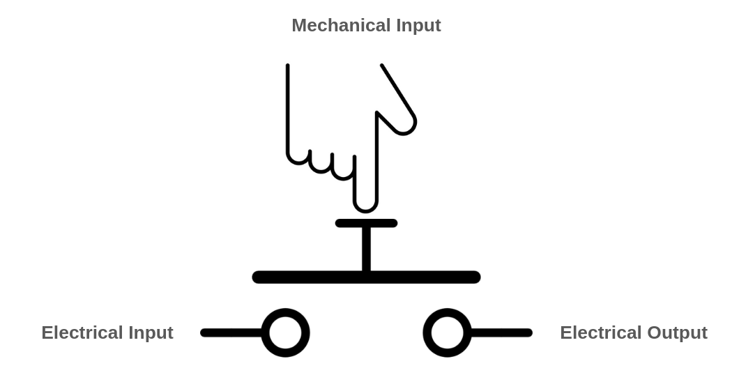
A simple example of a multi-input/single-output component is a switch. A switch controls the flow of an input to an output through a third, controlling input. Light switches, push buttons, and faucets (which control the flow of water through a pipe) are all examples of switches. However, in these cases, the type of the controlling input is different from the other inputs and outputs. For instance, the controlling input of a push button is mechanical, while the others are electrical. You still need a finger to push the button, and the output of the push button cannot be used as the mechanical input of another button. As a result, you can't build domino-like structures or long-lasting cause-and-effect chains using faucets or push buttons in the same way you would with purely similar types of inputs and outputs!
 { width=350px }
A push-button becomes more interesting when its controlling input is electrical rather than mechanical. In this case, all of its inputs and outputs are of the same type, allowing you to connect the output of one push-button to the controlling input of another.
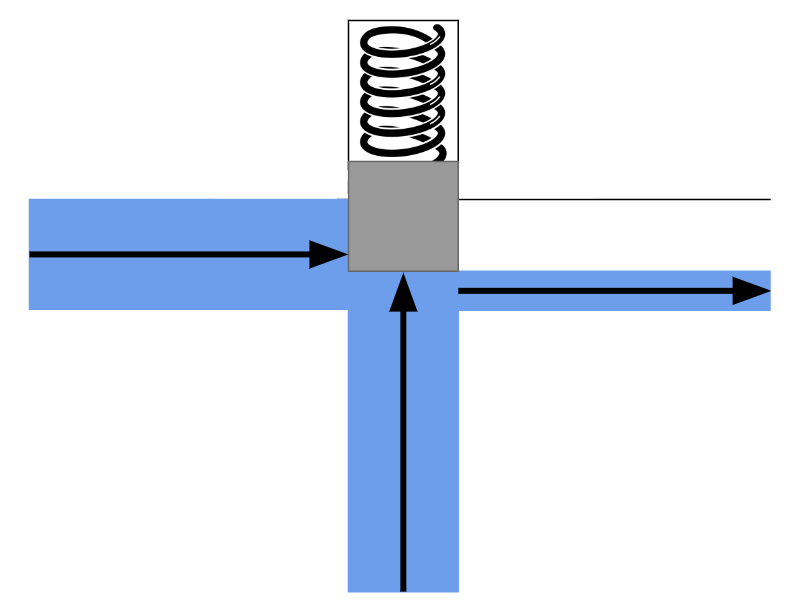
Similarly, in the faucet example, you could design a special kind of faucet that opens with the force of water, rather than requiring a person to open it manually with their hands. In the picture below, when no water is present in the controlling pipe (the pipe in the middle), the spring will push the block down, preventing water from flowing from the left pipe to the right pipe. However, when water enters the controlling pipe, its pressure will push the block up, creating space for the water to flow from the left pipe to the right pipe.
 { width=350px }
The controlling input doesn't have to sharply switch the flow between no-flow and maximum-flow. Instead, the controller can adjust the flow to any level, depending on how much the controlling input is pushed. Additionally, the controlling input doesn't need to be as large or powerful as the other inputs/outputs. It could be a thinner pipe that requires only a small force of water to fully open the valve. This means you can control a large and powerful water flow using a much smaller input and less force.
There’s also a well-known name for these unique switches: transistors. Now you can understand what "transistor" literally means—it’s something that can "transfer" or adjust "resistance" on demand, much like how we can control the resistance of the water flow in a larger pipe using a third input.
The most obvious use case for a transistor is signal amplification. Let’s explore this with an example: imagine a small pipe through which water flows in a sinusoidal pattern. Initially, there is no water, then the flow gradually increases to a certain level, and finally, it slowly decreases back to zero (a pattern similar to what you might see in a water show!). Now, we connect this pipe to the controlling input of the water transistor we designed earlier. Can you guess what comes out from the output of this transistor? Yes, the output is also a sinusoidal flow of water. The difference is that it’s much more powerful than the small pipe. We’ve just transferred the sinusoidal pattern from a small water flow to a much more powerful one! Can you imagine how important this is? This concept forms the core of how devices like electric guitars and sound amplifiers work!
That’s not the only use case for transistors, though. Because the cause-and-effect types of the inputs and outputs are the same, we can chain them together—and that’s all we need to start building machines that can compute things (we’ll explore the details soon!). These inputs don’t necessarily have to be electrical; they can be mechanical as well. Yes, we can build computers that operate using the force of water!
A typical transistor in the real world is conceptually the same as our imaginary faucet described above. Substitute water with electrons, and you have an accurate analogy for a transistor. Transistors, the building blocks of modern computers, allow you to control the flow of electrons in a wire using a third source of electrons!
Understanding how modern electron-based transistors work involves a fair bit of physics and chemistry. But if you insist, here’s a very simple (and admittedly silly) example of a push-button with an electrical controller: Imagine a person holding a wire in their hand. This person presses the push-button whenever they feel electricity in their hand (as long as the electricity isn’t strong enough to harm them). Together, the person and the push-button form something akin to a transistor, because now the types of all inputs and outputs in the system are the same.
It might sound like the strangest idea in the world, but if you had enough of these "transistors" connected together, you could theoretically build a computer capable of connecting to the internet and rendering webpages!
Why did people choose electrons to flow in the veins of our computers instead of something like water? There are several reasons:
- Electrons are extremely small.
- Electrical effects propagate extremely fast!
Thanks to these properties, we can create complex and dense cause-and-effect chains that produce amazing behaviors while using very little space, like in your smartphone!
Taming the electrons
In the previous section, we explored what a transistor is. Now it’s time to see what we can do with it! To quickly experiment with transistors, we’ll simulate imaginary transistors on a computer and arrange them in the right order to perform fancy computations for us.
Our ultimate goal is to construct a fully functional computer using a collection of three-way switches. If you have prior experience designing hardware, you're likely familiar with software tools that allow you to describe hardware using a Hardware Description Language (HDL). These tools can generate transistor-level circuits from your designs and even simulate them for you. However, since this book focuses on the underlying concepts rather than real-world, production-ready implementations, we will skip the complexity of learning an HDL. Instead, we'll use the Python programming language to emulate these concepts as we progress. This approach will not only deepen our understanding of the transistor-level implementation of something as intricate as a computer but also shed light on how HDL languages transform high-level circuit descriptions into collections of transistors.
So let's begin and start building our own circuit simulator!
Everything is relative
The very first term you encounter when exploring electricity is "voltage," so it’s essential to grasp its meaning before studying how transistors behave under different voltages. Formally, voltage is the potential energy difference between two points in a circuit. To understand this concept, let’s set aside electricity for a moment and think about heights.
Imagine lifting a heavy object from the ground. The higher you lift it, the more energy you expend (and the more tired you feel, right? That energy needs to be replenished, like by eating food!). According to the law of conservation of energy, energy cannot be created or destroyed, only transformed or transferred. So where does the energy you used to lift the object go?
Now, release the object and let it fall. It hits the ground with a bang, possibly breaking the ground—or itself. The higher the object was lifted, the greater the damage it causes. Clearly, energy is needed to create those noises and damages. But where did that energy come from?
You’ve guessed it! When you lifted the object, you transferred energy to it. When you let it fall, that stored energy was released. Physicists call this stored energy "potential energy." A raised object has the potential to do work (work is the result of energy being consumed), which is why it’s called potential energy!
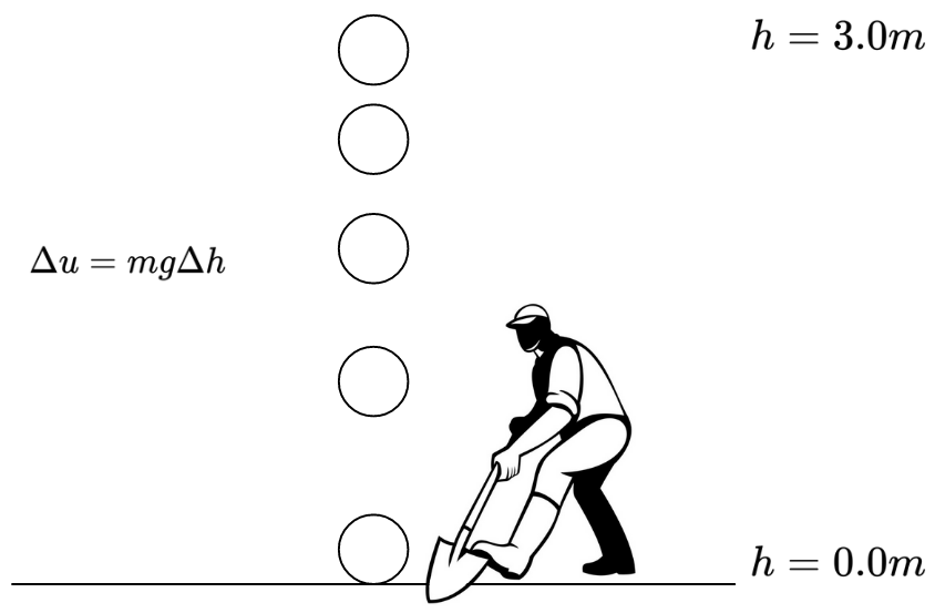
If you remember high school physics, you’ll know that the potential energy of an object can be calculated using the formula: \(U=mgh\), where \(m\) is the mass of the object, \(h\) is its height above the ground, and \(g\) is the Earth's gravitational constant (approximately \(9.807 m/s^2\)).
According to this formula, when the object is on the ground (\(h=0\)), the potential energy is also \(U=0\). But here’s an important question: does that mean an object lying on the ground has no potential energy?
Actually, it does have potential energy! Imagine taking a shovel and digging a hole under the object. The object would fall into the hole, demonstrating that it still had the capacity to do work due to gravity.
The key point is this: the equation \(U=mgh\) represents the potential energy difference relative to a chosen reference point (in this case, the ground), not the absolute potential energy of the object. A more precise way to express this idea would be: \(\varDelta{u}=mg\varDelta{h}\).
This equation shows that the potential energy difference between two points \(A\) and \(B\) depends on \(mg\), the gravitational force, and \(\varDelta{h}\), the difference in height between the two points.
In essence, potential energy is relative!
 { width=350px }
The reason it takes energy to lift an object is rooted in the fact that massive bodies attract each other, as described by the universal law of gravitation: \(F=G\frac{m_1m_2}{r^2}\).
Similarly, a comparable law exists in the microscopic world, where electrons attract protons, and like charges repel each other. This interaction is governed by Coulomb's law: \(F=k_e\frac{q_1q_2}{r^2}\)
As a result, we also have the concept of "potential energy" in the electromagnetic world. It takes energy to separate two electric charges of opposite types (positive and negative), as you're working against the attractive electric force. When you pull them apart and then release them, they will move back toward each other, releasing the stored potential energy.
That's essentially how batteries work. They create potential differences by moving electrons to higher "heights" of potential energy. When you connect a wire from the negative pole of the battery to the positive pole, the electrons "fall" through the wire, releasing energy in the process.
When we talk about "voltage," we are referring to the difference in height or potential energy between two points. While we might not know the absolute potential energy of points A and B, we can definitely measure and understand the difference in potential (voltage) between them!
Pipes of electrons
We discussed that transistors are essentially three-way switches that control the flow between two input/output paths using a third input. When building a transistor circuit simulator—whether simulating the flow of water or electrons—it makes sense to begin by simulating the "pipes," the elements through which electrons will flow. In electrical circuits, these "pipes" are commonly referred to as wires.
Wires are likely to be the most fundamental and essential components of our circuit simulation software. As their name suggests, wires are conductors of electricity, typically made of metal, that allow different components to connect and communicate via the flow of electricity. We can think of wires as containers that hold electrons at specific voltage levels. If two wires with different voltage levels are connected, electrons will flow from the wire with higher voltage to the one with lower voltage.
In digital circuits, transistors and other electronic components operate using two specific voltage levels: "zero" (commonly referred to as ground) and "one." It’s important to emphasize that the terms "zero" and "one" do not correspond to fixed or absolute values. Instead, "zero" acts as a reference point, while "one" represents a voltage level that is higher relative to "zero."
At first glance, it might seem that we could model a wire using a single boolean value: false to represent zero and true to represent one. However, this approach fails to account for all the possible scenarios that can arise in a circuit simulator.
For example, consider a wire in your simulator that isn’t connected to either the positive or negative pole of a battery. Would it even have a voltage level? Clearly, it would be neither 0 nor 1. Now imagine a wire that connects a high-voltage (1) wire to a low-voltage (0) wire. What would the voltage of this intermediary wire be? Electrons would start flowing from the higher-voltage wire to the lower-voltage wire, and as a result, the voltage of the intermediary wire would settle somewhere between 0 and 1.
In a digital circuit, connecting a 0 wire to a 1 wire is not always a good idea and could indicate a mistake in your circuit design, potentially causing a short circuit. Therefore, it is useful to consider a value for a wire that is either mistakenly or intentionally left unconnected (Free state) or connected to both 0 and 1 voltage sources simultaneously (Short-circuit/Unknown state).
Based on this explanation, a wire can be in four different states:
Zstate - The wire is free and not connected to anything.0state - The wire is connected to a ground voltage source and has 0 voltage.1state - The wire is connected to a 5.0V voltage source.Xstate - The wire's voltage cannot be determined because it is connected to both a 5.0V and 0.0V voltage source simultaneously.
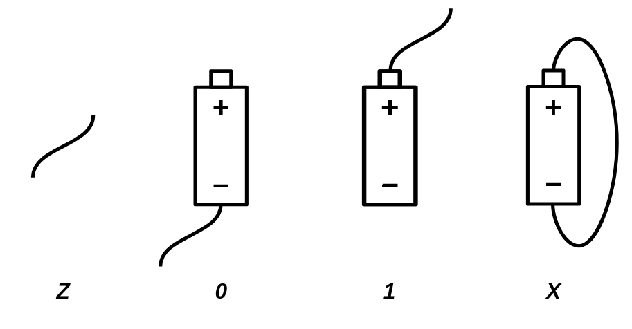
Initially, a wire that is not connected to anything is in the Z state. When you connect it to a gate or wire that has a state of 1, the wire's state will also become 1. A wire can connect to multiple gates or wires at the same time. For example, if a wire already in the 1 state is connected to another source of 1, it will remain 1. However, the wire will enter the X state if it is connected to a wire or gate with a conflicting value. For instance, if the wire is connected to both 0 and 1 voltage sources simultaneously, its state will be X. Similarly, connecting any wire to an X voltage source will also result in the wire taking on the X state.
We can summarize all the possible scenarios in a custom table that defines the arithmetic of wire states:
| A | B | A + B |
|---|---|---|
| Z | Z | Z |
| 0 | Z | 0 |
| 1 | Z | 1 |
| X | Z | X |
| Z | 0 | 0 |
| 0 | 0 | 0 |
| 1 | 0 | X |
| X | 0 | X |
| Z | 1 | 1 |
| 0 | 1 | X |
| 1 | 1 | 1 |
| X | 1 | X |
| Z | X | X |
| 0 | X | X |
| 1 | X | X |
| X | X | X |
A wildcard version of this table would look like this:
| A | B | A + B |
|---|---|---|
| Z | x | x |
| x | Z | x |
| X | x | X |
| x | X | X |
| 0 | 0 | 0 |
| 1 | 1 | 1 |
| 0 | 1 | X |
| 1 | 0 | X |
Based on the explanation, we can model a wire as a Python class:
FREE = "Z"
UNK = "X"
ZERO = 0
ONE = 1


class Wire:
    def __init__(self):
        self._drivers = {}
        self._assume = FREE

    def assume(self, val):
        self._assume = val

    def get(self):
        curr = FREE
        for b in self._drivers.values():
            if b == UNK:
                return UNK
            elif b != FREE:
                if curr == FREE:
                    curr = b
                elif b != curr:
                    return UNK
        return curr if curr != FREE else self._assume

    def put(self, driver, value):
        is_changed = self._drivers.get(driver) != value
        self._drivers[driver] = value
        return is_changed
The code above models a wire as a Python class. By definition, a wire that is not connected to anything remains in the Z state. Using the put function, a driver (such as a battery or a gate) can apply a voltage to the wire. The final voltage of the wire is determined by iterating over all the voltages applied to it.
We store the voltage values applied to the wire in a dictionary to ensure that a single driver cannot apply two different values to the same wire.
The put function also checks whether there has been a change in the values applied to the wire. This will later help our simulator determine if the circuit has reached a stable state, where the values of all wires remain fixed.
In some cases—particularly in circuits containing feedback loops and recursion—it is necessary to assume that a wire already has a value in order to converge on a solution. For this purpose, we have designed the assume() function, which allows us to assign an assumed value to a wire if no gates have driven a value into it. If you don’t yet fully understand what the assume() function does, don’t worry—we’ll explore its usage in the next sections.
Magical switches
Now that we've successfully modeled wires, it's time to implement the second most important component of our simulator: the transistor.
Transistors are electrically controlled switches with three pins: base, emitter, and collector. These pins connect to other circuit elements through wires. The base pin acts as the switch’s controller—when there is a high potential difference between the base and collector pins, the emitter connects to the collector. Otherwise, the emitter remains unconnected, behaving like a floating wire in the Z state.
This key behavior means that turning off the transistor does not set the emitter to 0 but instead leaves it in the Z state.
We can also describe the wire arithmetic of a transistor using the following table:
| B | E | C |
|---|---|---|
| 0 | 0 | Z |
| 0 | 1 | Z |
| 1 | 0 | 0 (Strong) |
| 1 | 1 | 1 (Weak) |
The transistor we have been discussing so far is a Type-N transistor. The Type-N transistor turns on when the base wire is driven with a 1. There is also another type of transistor, known as Type-P, which turns on when the base wire is driven with a 0. The truth table for a Type-P transistor looks like this:
| B | E | C |
|---|---|---|
| 0 | 0 | 0 (Weak) |
| 0 | 1 | 1 (Strong) |
| 1 | 0 | Z |
| 1 | 1 | Z |
Assuming we define a voltage of 5.0V as 1 and a voltage of 0.0V as 0, a wire is driven with a strong 0 when its voltage is very close to 0 (e.g., 0.2V), and a strong 1 when its voltage is close to 5 (e.g., 4.8V). The truth is, the transistors we build in the real world aren't ideal, so they won't always provide strong signals. A signal is considered weak when it's far from 0.0V or 5.0V. For example, a voltage of 4.0V could be considered a weak 1, and a voltage of 1.0V would be considered a weak 0, whereas 4.7V could be considered a strong 1 and 0.3V a strong 0. Type-P transistors, when built in the real world, are very good at producing strong 0 signals, but their 1 signals tend to be weak. On the other hand, Type-N transistors produce strong 1 signals, but their 0 signals are weak. By using both types of transistors together, we can build logic gates that provide strong outputs in all cases.
The Transistor
In our digital circuit simulator, we’ll have two different types of components: primitive components and components that are made of primitives. We’ll define components as primitives when they can’t be described as a group of smaller primitives.
For example, we can simulate Type-N and Type-P transistors as primitive components, since everything else can be constructed by combining Type-N and Type-P transistors together.
class NTransistor:
    def __init__(self, in_base, in_collector, out_emitter):
        self.in_base = in_base
        self.in_collector = in_collector
        self.out_emitter = out_emitter

    def update(self):
        b = self.in_base.get()
        if b == ONE:
            return self.out_emitter.put(self, self.in_collector.get())
        elif b == ZERO:
            return self.out_emitter.put(self, FREE)
        elif b == UNK:
            return self.out_emitter.put(self, UNK)
        else:
            return True  # Trigger re-update


class PTransistor:
    def __init__(self, in_base, in_collector, out_emitter):
        self.in_base = in_base
        self.in_collector = in_collector
        self.out_emitter = out_emitter

    def update(self):
        b = self.in_base.get()
        if b == ZERO:
            return self.out_emitter.put(self, self.in_collector.get())
        elif b == ONE:
            return self.out_emitter.put(self, FREE)
        elif b == UNK:
            return self.out_emitter.put(self, UNK)
        else:
            return True  # Trigger re-update
Our primitive components are classes with an update() function. The update() function is called whenever we want to calculate the output of the primitive based on its inputs. As a convention, we will prefix the input and output wires of our components with in_ and out_, respectively.
The update() function of our primitive components will also return a boolean value, which indicates whether the element needs to be updated again. Sometimes, the inputs of a component might not be ready when the update() function is called. For example, in the case of transistors, if the base wire is in the Z state, we assume there is another transistor that needs to be updated before the current transistor can calculate its output. By returning this boolean value, we inform our circuit emulator that the transistor is not "finalized" yet, and the update() function needs to be called again before determining that all component outputs have been correctly calculated and the circuit is stabilized.
Additionally, remember that the put() function of the Wire class also returns a boolean value. This value indicates whether the driver of that wire has placed a new value on the wire. A new value on a wire means there has been a change in the circuit, and the entire circuit needs to be updated again.
The Circuit
Now, it would be useful to have a data structure for keeping track of the wires and transistors allocated in a circuit. We will call this class Circuit. It will provide methods for creating wires and adding transistors. The Circuit class is responsible for calling the update() function of the primitive components and will allow you to calculate the values of all the wires in the network.
class Circuit:
    def __init__(self):
        self._wires = []
        self._comps = []

        self._zero = self.new_wire()
        self._zero.put(self, ZERO)
        self._one = self.new_wire()
        self._one.put(self, ONE)

    def one(self):
        return self._one

    def zero(self):
        return self._zero

    def new_wire(self):
        w = Wire()
        self._wires.append(w)
        return w

    def add_component(self, comp):
        self._comps.append(comp)

    def num_components(self):
        return len(self._comps)

    def update(self):
        has_changes = False
        for t in self._comps:
            has_changes = has_changes | t.update()
        return has_changes

    def stabilize(self):
        while self.update():
            pass
The update() method of the Circuit class calculates the values of the wires by iterating through the transistors and calling their update method. In circuits with feedback loops, a single iteration of updates may not be sufficient, and multiple iterations may be needed before the circuit reaches a stable state. To address this, we introduce an additional method specifically designed for this purpose: stabilize(). This method repeatedly performs updates until no changes are observed in the wire values, meaning the circuit has stabilized.
Our Circuit class also provides global zero() and one() wires, which can be used by components requiring fixed 0 and 1 signals. These wires function like battery poles in our circuits.
Electronic components can be defined as functions that take a circuit as input and add wires and transistors to it. Let’s explore the implementation details of some of them!
Life in a non-ideal world
Digital circuits are essentially logical expressions that are automatically evaluated by the flow of electrons through what we refer to as gates. Logical expressions are defined using zeros and ones, but as we have seen, wires in an electronic circuit are not always guaranteed to be either 0 or 1. Therefore, we must redefine our gates and determine their output in cases where the inputs are faulty.
Consider a NOT gate as an example. In an ideal world, its truth table would be as follows:
| A | NOT A |
|---|---|
| 0 | 1 |
| 1 | 0 |
However, the real world is not ideal, and wires connected to electronic logic gates can have unexpected voltages. Since a wire in our emulation can have four different states, our logic gates must be able to handle all four. The following is the definition of a NOT gate using our wire arithmetic. If the input to the NOT gate is Z or X, the output will be the faulty state X.
| A | NOT A |
|---|---|
| 0 | 1 |
| 1 | 0 |
| Z | X |
| X | X |
There are two ways to simulate gates in our software. We can either implement them using plain Python code as primitive components, similar to transistors, or we can construct them as a circuit of transistors. The following is an example of a NOT gate implemented using the first approach:
class Not:
    def __init__(self, wire_in, wire_out):
        self.wire_in = wire_in
        self.wire_out = wire_out

    def update(self):
        v = self.wire_in.get()
        if v == FREE:
            self.wire_out.put(self, UNK)
        elif v == UNK:
            self.wire_out.put(self, UNK)
        elif v == ZERO:
            self.wire_out.put(self, ONE)
        elif v == ONE:
            self.wire_out.put(self, ZERO)
We can also test out implementation:
if __name__ == '__main__':
    inp = Wire.zero()
    out = Wire()
    gate = Not(inp, out)
    gate.update()
    print(out.get())
The NOT gate modeled as a primitive component is accurate and functions as expected. However, we know that a NOT gate is actually built from transistors, and it might be more interesting to model it using a pair of transistors rather than cheating by emulating its high-level behavior with Python code.
The following is an example of a NOT gate constructed using a P-type and an N-type transistor:
def Not(circuit, inp, out):
    circuit.add_component(PTransistor(inp, circuit.one(), out))
    circuit.add_component(NTransistor(inp, circuit.zero(), out))
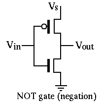
As you know, an N-type transistor connects its source pin to its drain pin when the voltage on its gate is higher than the voltage on its drain. So, when the inp wire is driven with 1, the output gets connected to the circuit.zero() wire, causing out to hold a 0 signal. Notice that the P-type transistor is off when inp is 1, so the circuit.one() wire will not get connected to the output pin. If that were the case, we would get a short circuit, causing the out signal to become a faulty (X)`.
Likewise, when inp is 0, the P-type transistor turns on and connects the output to circuit.one(), while the N-type transistor turns off, leaving the output unconnected to the ground.
NOT gates are probably the simplest components you can build using the current primitive elements provided by our simulator. Now that we’re familiar with transistors, it’s time to expand our component set and build some of the most fundamental logic gates. In addition to NOT gates, you’ve likely heard of AND and OR gates, which are a bit more complex—mainly because they take more than one input. Here’s their definition:
AND gate: outputs 0 when at least one of the inputs is 0, and gets 1 when all of the inputs are 1. Otherwise the output is faulty (X).
| A | B | A AND B |
|---|---|---|
| 0 | * | 0 |
| * | 0 | 0 |
| 1 | 1 | 1 |
| X |
OR gate: outputs 1 when at least one of the inputs is 1, and gets 0 only when all of the inputs are 0. Otherwise the output is unknown (X).
| A | B | A OR B |
|---|---|---|
| 1 | * | 1 |
| * | 1 | 1 |
| 0 | 0 | 0 |
| X |
Mother of the gates
A NAND gate is a logic gate that outputs 0 if and only if both of its inputs are 1. It is essentially an AND gate with its output inverted. It can be proven that all the basic logic gates (AND, OR, NOT) can be built using different combinations of this single gate:
- \(NOT(x) = NAND(x, x)\)
- \(AND(x, y) = NOT(NAND(x, y)) = NAND(NAND(x, y), NAND(x, y))\)
- \(OR(x, y) = NAND(NOT(x), NOT(y)) = NAND(NAND(x, x), NAND(y, y))\)
It is the "mother gate" of all logic circuits. Although building everything with NAND gates would be very inefficient in practice, for the sake of simplicity, we'll stick to NAND gates and try to construct other gates by connecting them together.

It turns out that we can build NAND gates with strong and accurate output signals using 4 transistors (2 Type-N and 2 Type-P). Let's prototype a NAND gate using our simulated N/P transistors!
def Nand(circuit, in_a, in_b, out):
    inter = circuit.new_wire()
    circuit.add_component(PTransistor(in_a, circuit.one(), out))
    circuit.add_component(PTransistor(in_b, circuit.one(), out))
    circuit.add_component(NTransistor(in_a, circuit.zero(), inter))
    circuit.add_component(NTransistor(in_b, inter, out))
Now, other primitive gates can be defined as combinations of NAND gates. Take the NOT gate as an example. Here is a third way we can implement a NOT gate (So far, we have implemented a NOT gate in two ways: 1. Describing its behavior through plain Python code, and 2. By connecting a pair of Type-N and Type-P transistors):
def Not(circuit, inp, out):
    Nand(circuit, inp, inp, out)
Go ahead and implement the other primitive gates using the NAND gate we just defined. After that, we can start creating useful circuits from these gates!
def And(circuit, in_a, in_b, out):
    not_out = circuit.new_wire()
    Nand(circuit, in_a, in_b, not_out)
    Not(circuit, not_out, out)


def Or(circuit, in_a, in_b, out):
    not_out = circuit.new_wire()
    Nor(circuit, in_a, in_b, not_out)
    Not(circuit, not_out, out)


def Nor(circuit, in_a, in_b, out):
    inter = circuit.new_wire()
    circuit.add_component(PTransistor(in_a, circuit.one(), inter))
    circuit.add_component(PTransistor(in_b, inter, out))
    circuit.add_component(NTransistor(in_a, circuit.zero(), out))
    circuit.add_component(NTransistor(in_b, circuit.zero(), out))
An XOR gate is another incredibly useful gate that comes in handy when building circuits that can perform numerical additions. The XOR gate outputs 1 only when the inputs are unequal, and outputs 0 when they are equal. XOR gates can be built from AND, OR, and NOT gates: \(Xor(x,y) = Or(And(x, Not(y)), And(Not(x), y))\). However, since XOR gates will be used frequently in our future circuits, it makes more sense to provide a transistor-level implementation for them, as this will require fewer transistors!
def Xor(circuit, in_a, in_b, out):
    a_not = circuit.new_wire()
    b_not = circuit.new_wire()
    Not(circuit, in_a, a_not)
    Not(circuit, in_b, b_not)

    inter1 = circuit.new_wire()
    circuit.add_component(PTransistor(b_not, circuit.one(), inter1))
    circuit.add_component(PTransistor(in_a, inter1, out))
    inter2 = circuit.new_wire()
    circuit.add_component(PTransistor(in_b, circuit.one(), inter2))
    circuit.add_component(PTransistor(a_not, inter2, out))

    inter3 = circuit.new_wire()
    circuit.add_component(NTransistor(in_b, circuit.zero(), inter3))
    circuit.add_component(NTransistor(in_a, inter3, out))
    inter4 = circuit.new_wire()
    circuit.add_component(NTransistor(b_not, circuit.zero(), inter4))
    circuit.add_component(NTransistor(a_not, inter4, out))
Sometimes, we simply need to connect two different wires. Instead of creating a new primitive component for that purpose, we can use two consecutive NOT gates. This will act like a simple jumper! We'll call this gate a Forward gate:
def Forward(circuit, inp, out):
    tmp = circuit.new_wire()
    Not(circuit, inp, tmp)
    Not(circuit, tmp, out)
Hello World circuit!
The simplest digital circuit we might consider a "computer" is one that can perform basic arithmetic, like adding two numbers together. In digital circuits, information is represented using binary signals—0s and 1s. So, when we talk about adding numbers in a digital circuit, we're working with binary numbers.
To start with, let's focus on a very basic example: a circuit that can add two one-bit binary numbers. A one-bit number can only be either a 0 or a 1, so adding them together can yield one of three possible results: 0 + 0 = 0, 0 + 1 = 1, and 1 + 1 = 10 (which is 2 in decimal). Notice that the result of adding two one-bit numbers is always a two-bit number, because 1 + 1 produces a carry, which means we need two bits to store the result.
To design such a circuit, one of the most effective approaches is to start by figuring out what the output should be for each possible combination of inputs. Since there are two inputs (each one-bit numbers), there are four possible input combinations: 00, 01, 10, and 11. For each of these combinations, we can determine what the output should be. Since the result is always a two-bit number, we can break the circuit into two smaller subcircuits: one that calculates the sum bit (the least significant bit) and one that calculates the carry bit (the more significant bit). Each subcircuit works independently to compute its corresponding part of the result.
In this way, we approach building the circuit step by step, using logic gates to implement the required operations for each input combination.
| A | B | First digit | Second digit |
|---|---|---|---|
| 0 | 0 | 0 | 0 |
| 0 | 1 | 1 | 0 |
| 1 | 0 | 1 | 0 |
| 1 | 1 | 0 | 1 |
The relation of the second digit with A and B is very familiar; it's essentially an AND gate! Try to figure out how the first digit can be calculated by combining primitive gates. (Hint: It outputs 1 only when A is 0 AND B is 1, or A is 1 AND B is 0.)
Answer: It's an XOR gate! (\(Xor(x, y) = Or(And(x, Not(y)), And(Not(x), y))\)), and here is the Python code for the entire thing:
def HalfAdder(circuit, in_a, in_b, out_sum, out_carry):
    Xor(circuit, in_a, in_b, out_sum)
    And(circuit, in_a, in_b, out_carry)
What we have just built is known as a half-adder. With a half-adder, you can add 1-bit numbers together. You might think that we can build multi-bit adders by stacking multiple half-adders in a row, but that's not entirely correct. Recall that the addition algorithm we learned in primary school also applies to binary numbers. Imagine we want to add the binary numbers 1011001 (89) and 111101 (61) together. Here’s how it works:
 1111  1

  1011001
+  111101
-----------
 10010110
By examining the algorithm, we can see that for each digit, the addition involves three bits (not just two). In addition to the original bits, there is also a third carry bit from the previous addition that must be considered. Therefore, to design a multi-bit adder, we need a circuit that can add three one-bit numbers together. Such a circuit is known as a full-adder, and the third number is often referred to as the carry bit. Here’s the truth table for a three-bit adder:
| A | B | C | D0 | D1 |
|---|---|---|---|---|
| 0 | 0 | 0 | 0 | 0 |
| 1 | 0 | 0 | 1 | 0 |
| 0 | 1 | 0 | 1 | 0 |
| 1 | 1 | 0 | 0 | 1 |
| 0 | 0 | 1 | 1 | 0 |
| 1 | 0 | 1 | 0 | 1 |
| 0 | 1 | 1 | 0 | 1 |
| 1 | 1 | 1 | 1 | 1 |
Building a full-adder is not that challenging. You can use two half-adders to compute the sum bit and then take the OR of the carry outputs to obtain the final carry bit.
def FullAdder(circuit, in_a, in_b, in_carry, out_sum, out_carry):
    sum_ab = circuit.new_wire()
    carry1 = circuit.new_wire()
    carry2 = circuit.new_wire()
    HalfAdder(circuit, in_a, in_b, sum_ab, carry1)
    HalfAdder(circuit, sum_ab, in_carry, out_sum, carry2)
    Or(circuit, carry1, carry2, out_carry)
Once we have a full-adder ready, we can proceed with building multi-bit adders. For example, to create an 8-bit adder, we need to connect eight full-adders in a row. The carry output of each adder serves as the carry input for the next, mimicking the addition algorithm we discussed earlier.
def Adder8(circuit, in_a, in_b, in_carry, out_sum, out_carry):
    carries = [in_carry] + [circuit.new_wire() for _ in range(7)] + [out_carry]
    for i in range(8):
        FullAdder(
            circuit,
            in_a[i],
            in_b[i],
            carries[i],
            out_sum[i],
            carries[i + 1],
        )
Congratulations! We just added two 8-bit numbers using nothing but bare transistors. Before continuing our journey toward more complex circuits, let's ensure that our simulated model of the 8-bit adder is functioning correctly. If the 8-bit adder works properly, there is a high chance that the other gates are also functioning as expected.
def num_to_wires(circuit, num):
    wires = []
    for i in range(8):
        bit = (num >> i) & 1
        wires.append(circuit.one() if bit else circuit.zero())
    return wires


def wires_to_num(wires):
    out = 0
    for i, w in enumerate(wires):
        if w.get() == ONE:
            out += 2**i
    return out


if __name__ == "__main__":
    for x in range(256):
        for y in range(256):
            circuit = Circuit()
            wires_x = num_to_wires(circuit, x)
            wires_y = num_to_wires(circuit, y)
            wires_out = [Wire() for _ in range(8)]
            Adder8(circuit, wires_x, wires_y, circuit.zero(), wires_out, circuit.zero())
            circuit.update()
            out = wires_to_num(wires_out)
            if out != (x + y) % 256:
                print("Adder is not working!")
Here, we are checking if the outputs are correct for all possible inputs. We have defined two auxiliary functions, num_to_wires and wires_to_num, to convert numbers into a set of wires that can connect to an electronic circuit, and vice versa.
When addition is subtraction
So far, we have been able to implement the addition operation by combining N and P transistors. Our adder is limited to 8 bits, meaning that the input and output values are all in the range \([0,255]\). If you try to add two numbers whose sum exceeds 255, you will still get a result in the range \([0,255]\). This happens because a number larger than 255 cannot be represented by 8 bits, and an overflow occurs. Upon closer inspection, you’ll notice that what we have designed isn’t the typical addition operation we are used to in elementary school mathematics; instead, it’s addition in a finite field. This means the addition results are taken modulo 256.
\(a \oplus b = (a + b) \mod 256\)
It is good to know that finite-fields have interesting properties:
- \((a \oplus b) \oplus c = a \oplus (b \oplus c)\)
- For every non-zero number \(x \in \mathbb{F}\), there is a number \(y\), where \(x \oplus y = 0\). \(y\) is known as the negative of \(x\).
In a finite field, the negative of a number can be calculated by subtracting that number from the field size (in this case, the size of our field is \(2^8=256\)). For example, the negative of \(10\) is \(256-10=246\), so \(10 \oplus 246 = 0\).
Surprisingly, the number \(246\), behaves exactly like \(-10\). Try adding \(246\) to \(15\). You will get \(246 \oplus 15 = 5\) which is the same as \(15 + (-10)\)! This has an important implication: we can perform subtraction without designing a new circuit! All we need to do is negate the number. Calculating the negative of a number is like taking the XOR of that number (Which gives \(255 - a\)), and then adding \(1\) to it (Which results in \(256 - a\), our definition of negation). This is known as the two's complement form of a number.
It’s incredible to see that we can build electronic machines capable of adding and subtracting numbers by simply connecting a bunch of transistors together! The good news is that we can go even further and design circuits that can perform multiplication and division, using the same approach we used for designing addition circuits. The details of multiplication and division circuits are beyond the scope of this book, but you are strongly encouraged to study them on your own!
Not gates can be fun too!
If you remember, we discussed that you can't build interesting structures using only a single type of single-input/single-output component (such as NOT gates). In fact, we argued that using just them, we can only create domino-like structures, where a single cause traverses through the components until reaching the last one. However, that's not entirely true: what if we connect the last component of the chain to the first one? This creates a loop, which is definitely something new. Assuming two consecutive NOT gates cancel each other out, we can build two different kinds of NOT loops:
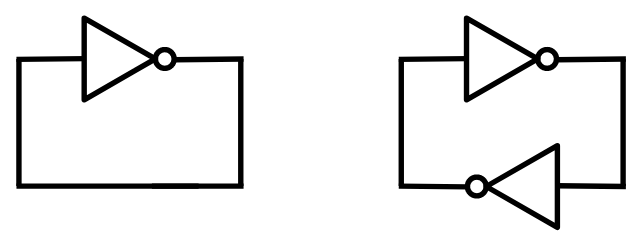
After analyzing both possible loops, you will soon understand that the one with a single NOT gate is unstable. The voltage of the wire can be neither 0 nor 1. It creates a logical paradox, similar to the statement: This sentence is not true. The statement can be neither true nor false!
Practically, if you build such a circuit, it may oscillate rapidly between possible states, or the wire's voltage may settle at a value between the logical voltages of 0 and 1.
On the other hand, the loop with two NOT gates can achieve stability. The resulting circuit has two possible states: either the first wire is 1 and the second wire is 0, or the first wire is 0 and the second wire is 1. It will not switch between these states automatically. If you build such a circuit using real components, the initial state will be somewhat random. A slight difference in the transistor conditions may cause the circuit to settle into one of the states and remain there.
Try to remember
So far, we have been experimenting with stateless circuits—circuits that do not need to store or remember anything to function. However, circuits without memory are severely limited in their capabilities. To unlock their full potential, we need to explore how to store data within a digital circuit and maintain it over time. This is one of the most critical steps before we can build a computer, as computers are essentially machines that manipulate values stored in some kind of memory. Without memory, a computer cannot perform complex tasks or execute meaningful programs.
As a child, you may have tried to leave a light switch in a "middle" position. If the switch was well-made, you probably found it frustratingly difficult to do! The concept of memory arises when a system with multiple possible states can only stabilize in a single state at a time. Once it becomes stable, it can only change through an external force. In this sense, a light switch can function as a single-bit memory cell.
Another silly example: imagine a piece of paper—it remains stable in its current state. If you set it on fire, it gradually changes until it is completely burned, after which it stabilizes again. Keeping the paper in a "half-burned" state is not easy! You could consider the paper as a crude single-bit memory cell, but it has a major flaw: once burned, it cannot return to its original state.
Fortunately, there are ways to build circuits with multiple possible states, where only one state remains stable at a time. The simplest example is a circuit that forms a loop by connecting two NOT gates to each other. This setup involves two wires: if the first wire is 1, the second wire will be 0, and the circuit will stabilize in that configuration (and vice versa).
The problem with a simple NOT gate loop is that it cannot be controlled externally—it lacks an input mechanism to change its state. To fix this, we can replace the NOT gates with logic gates that accept two inputs instead of one. For example, using NAND gates instead allows us to introduce external control. By providing voltages to the extra input pins, a user can modify the internal state of the loop. This type of circuit is known as an SR latch:
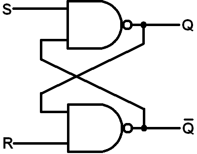
Now, the user can set the latch to the first or second state by setting S=1 and R=0, or S=0 and R=1, respectively. The magic lies in the fact that the circuit will stably remain in the latest state, even after both S and R inputs are set to zero!
Here you can find an example of a SR latch implemented in Python:
def SRLatch(circuit, in_r, in_s, out_data, initial=0):
    neg_out = circuit.new_wire()
    Nor(circuit, in_r, neg_out, out_data)
    Nor(circuit, in_s, out_data, neg_out)
    neg_out.assume(1 - initial)
    out_data.assume(initial)
Notice how we ingeniously feed two set/reset inputs into something that is essentially a NOT loop! Now, there’s something tricky about simulating a NOR/NOT loop: How can the first NOR gate function when neg_out is still not calculated? Or similarly, how can the second NOR gate calculate neg_out when out_data is still not calculated? There are two approaches we can use to resolve the chicken-and-egg problem in our simulation:
- Give up and attempt to simulate a memory-cell component without performing low-level transistor simulations. This would require us to define a new Primitive Component (similar to N/P transistors), which includes an
update()function that mimics the expected behavior of a latch. - Hint the simulator with the initial values of wires, and let the simulator to settle in an stable state by running the update function of the transistors for a few iterations and stopping the iterations after the wire values stop changing (Meaning that the system has entered a stable state).
That’s where the assume function we defined for our Wire class comes in handy. The assume function essentially hints to the simulator the initial value(s) of the wires in our memory cell, making it stable. In fact, if you don’t call these assume functions when defining the gates, the simulator won’t be able to simulate it, and the output of both NOR gates would become X. Assumption is only necessary when we want to initialize the circuit in a stable state for the first time. After that, the circuit will ignore the initial assumed values and will start working as expected. Note: In the real world, the memory cell randomly settles into one of the set/reset states due to environmental noise and slight differences between the transistors.
A more user-friendly latch
SR latches are perfect examples of memory cells since they can store a single bit of data. However, the unusual aspect of SR latches is that they require two inputs to determine whether to set them to a set (1) or reset (0) state. To set the latch to a 1 (set) state, you would feed it S=1 & R=0, and to reset it to 0 (reset) state, you would feed it S=0 & R=1. But what if we only had a single wire, D=0/1, and wanted the latch to remember the value stored in that wire? This is where the D-latch, a second type of latch, comes in handy.
Building a D-latch is quite straightforward: you simply need to create a circuit that decodes a single D bit into two S and R bits. The circuit should output SR=01 when D=0 and SR=10 when D=1. This circuit is essentially a 1x2 decoder, which can then be connected to your existing SR-latch.
There’s a problem when we simply connect a 2x1 decoder to an SR latch: how can we tell the latch to stop copying whatever value is present on the D wire into its internal state? In an SR latch, the answer is straightforward: when both S and R are set to 0, the latch’s internal state won’t change and will simply remain in its most recent state. We would like to have the same kind of control in a D-latch, or else the D-latch would be no different than a simple wire! To achieve this, we introduce a new control wire called clock (or clk), which stops the latch from acquiring the value of D. The truth table for such a circuit would look something like this:
| Previous state | CLK | D | Next state |
|---|---|---|---|
| 0 | 0 | 0 | 0 |
| 0 | 0 | 1 | 0 |
| 0 | 1 | 0 | 0 |
| 0 | 1 | 1 | 1 |
| 1 | 0 | 0 | 1 |
| 1 | 0 | 1 | 1 |
| 1 | 1 | 0 | 0 |
| 1 | 1 | 1 | 1 |
Here is how the schematic representation of a D-latch would look:
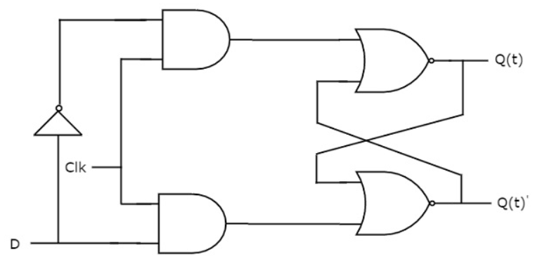
And how it can be represented with our Python simulator:
def DLatch(circuit, in_clk, in_data, out_data, initial=0):
    not_data = circuit.new_wire()
    Not(circuit, in_data, not_data)
    and_d_clk = circuit.new_wire()
    And(circuit, in_data, in_clk, and_d_clk)
    and_notd_clk = circuit.new_wire()
    And(circuit, not_data, in_clk, and_notd_clk)
    neg_out = circuit.new_wire()
    Nor(circuit, and_notd_clk, neg_out, out_data)
    Nor(circuit, and_d_clk, out_data, neg_out)

    neg_out.assume(1 - initial)
    out_data.assume(initial)
Later in this book, we will be building a computer with memory cells of size 8 bits (a.k.a. a byte). It might make sense to group 8 of these DLatches together as a separate component in order to build our memory cells, registers, and RAM. We'll need to arrange the latches in a row and connect their enable pins together. The resulting component will have 9 input wires (1-bit in_clk and 8-bit in_data) and 8 output wires (8-bit out_data):
class Reg8:
    def snapshot(self):
        return wires_to_num(self.out_data)

    def __init__(self, circuit, in_clk, in_data, out_data, initial=0):
        self.out_data = out_data
        for i in range(8):
            DLatch(  # WARN: A DLatch may not be appropriate here...
                circuit,
                in_clk,
                in_data[i],
                out_data[i],
                ZERO if initial % 2 == 0 else ONE,
            )
            initial //= 2
There is something wrong with this register component. Let's discover the problem in action!
Make it count!
Since we now know how to build memory cells, we can create circuits that maintain state/memory and behave accordingly! Let's build something useful with it!
A very simple yet useful stateful circuit you can build, using adders and memory cells, is a counter. An 8-bit counter can be made by taking the output of an 8-bit memory cell, incrementing it, and then feeding it back to the input of the memory cell. In this case, we expect the value of the counter to be incremented every time the clock signal rises and falls. Here’s what the Python simulator for an 8-bit counter would look like. Try running it, and you’ll see that the simulator gets stuck and is unable to stabilize!
class Counter:
    def snapshot(self):
        print("Value:", self.counter.snapshot())

    def __init__(self, circuit: Circuit, in_clk: Wire):
        one = [circuit.one()] + [circuit.zero()] * 7

        counter_val = [circuit.new_wire() for _ in range(8)]
        next_counter_val = [circuit.new_wire() for _ in range(8)]

        Adder8(
            circuit,
            counter_val,
            one,
            circuit.zero(),
            next_counter_val,
            circuit.new_wire(),
        )

        self.counter = Reg8(circuit, in_clk, next_counter_val, counter_val, 0)


if __name__ == "__main__":
    circ = Circuit()
    clk = circ.new_wire()

    OSCILLATOR = "OSCILLATOR"

    clk.put(OSCILLATOR, ZERO)

    counter = Counter(circ, clk)
    print("Num components:", circ.num_components())

    while True:
        circ.stabilize()  # WARN: Gets stuck here!
        counter.snapshot()
        clk.put(OSCILLATOR, 1 - clk.get())
When you think about it, the reason the circuit doesn’t stabilize becomes clear: as soon as the clock signal rises to 1, the feedback loop activates and continues to operate as long as the clock remains at 1. However, the clock signal stays at 1 for a certain period before dropping back down to 0. During that time, the circuit keeps trying to increment the value of the memory cell, which prevents it from stabilizing. We introduced the clock signal to allow us to control our stateful circuit as it iterates through different states, but it seems that a DLatch isn't giving us the control we need.
In fact, the enable input of the D-Latch (the clock signal) should be set to 1 for only a very short time—we just need a brief tick. Otherwise, the circuit will enter an unstable state. As soon as the input of the memory cell is captured, the output will change shortly after. If the enable signal is still 1, the circuit will continue incrementing and updating its internal state. The duration for which the enable signal is 1 should be short enough that the incrementor component doesn't have enough time to update its output, Otherwise, our circuit will be no different from connecting the output of a NOT gate to its input, in terms of instability!
A straightforward idea for solving the problem is to make the time the clock stays high short enough to resemble a pulse—just long enough to let the circuit transition to its next state, but not so long that it starts looping and becomes unstable. One way to create such pulses is by passing a typical clock signal through an edge detector. An edge detector is an electronic circuit that can recognize sharp changes in a signal.
So, how can we build an edge detector? There's an interesting twist in the real world that we can exploit: because logic gates have propagation delays, unusual behaviors—known as hazards—can occur. These are brief, unintended outputs caused by timing mismatches in signal changes.
Consider this example circuit:
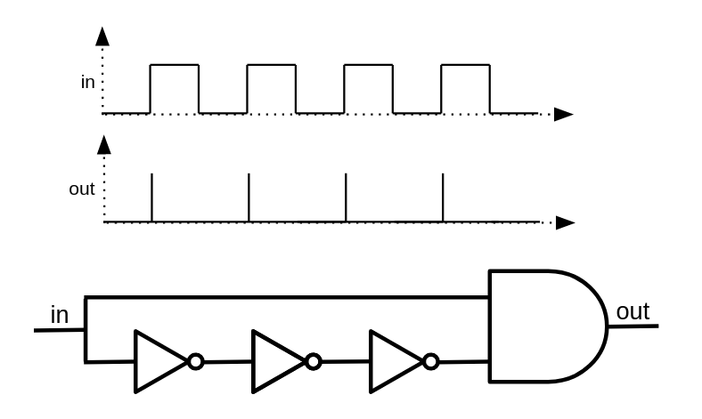
When the input is 0, the NOT gate outputs 1. Now, when the input switches to 1, the wire that goes directly to the AND gate receives 1 immediately. However, the wire that goes through the NOT gate takes a brief moment to reflect the change, still holding 1 for a short time before it becomes 0. During that brief moment, both inputs of the AND gate are 1, causing it to produce a short, unintended high output—a glitch or pulse.
By closely observing the behavior of this circuit, we can see that it effectively converts a clock signal into a train of ultra-short pulses. If we connect this component to the enable pin of a latch, the latch will update only on the rising edge of the clock signal. This configuration is known as a flip-flop.
The only difference between a flip-flop and a latch is in how they respond to the clock: flip-flops are edge-triggered, while latches are level-triggered. Flip-flops are preferred when designing synchronous circuits, as they provide better timing control and predictability.
Unfortunately, our digital circuit simulator is not a perfect representation of the real world. Since it doesn't account for gate delays, we can't build edge detectors as we discussed earlier. Even if we could, it wouldn't be a very clean solution for someone like me, who tends to be a bit paranoid. Just imagine if one of those pulses happens to be shorter or longer than expected—it could break the entire computation!
Fortunately, there's a cleaner and more reliable way to solve the looping problem, one that doesn’t rely on exploiting subtle physical behaviors. It starts by breaking the loop through serially connecting two D-latches: one that activates when the clock signal goes low, and the other when the clock signal goes high. This way, there is no point in time when both latches are active, so a loop can't form, even though data is still being reliably stored. Curious why it's called a flip-flop? When the clock signal rises, the first D-latch gets activated and it "flips." Then, when the clock signal falls, the first latch becomes inactive, the second latch activates, and it "flops!" And just like that, we form a flip-flop!
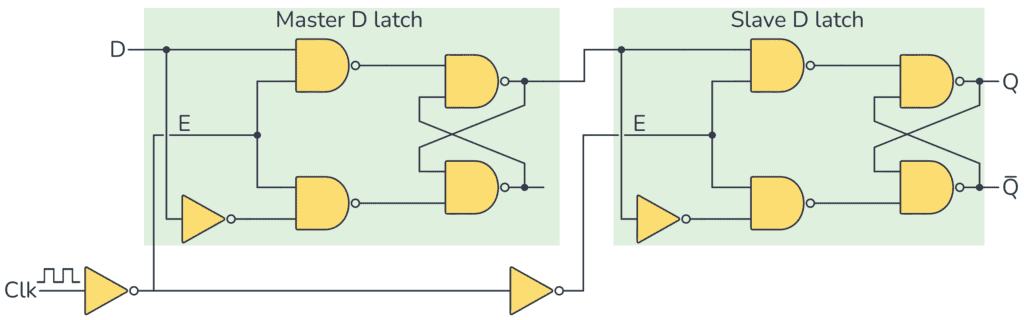
Here's the Python implementation of the structure we just described:
def DFlipFlop(circuit, in_clk, in_data, out_data, initial=0):
    neg_clk = circuit.new_wire()
    Not(circuit, in_clk, neg_clk)
    inter = circuit.new_wire()
    DLatch(circuit, in_clk, in_data, inter, initial)
    DLatch(circuit, neg_clk, inter, out_data, initial)
In our Counter circuit example, substitute the registers we built with DLatches with ones built using DFlipFlops, and the stabilization problem is solved!
Counters on steroids!
A counter circuit is a perfect example of how digital circuits can remember their state and transition to a new state in a controlled fashion. It’s also a fundamental concept that inspires us to build much more complex systems, including computers.
A computer, in its simplest form, consists of memory, which stores all instructions and data, and a CPU, which fetches and interprets them. Looking closely at the whole system, you can see that the CPU/memory pair is not very different from the register/incrementer pair in a counter circuit. There is a state (in the counter circuit, a single byte within a register; in the computer, several billion memory cells), and there is a state manipulator (in the counter circuit, an incrementer; in the computer, a component that decodes the current instruction and executes it). On every clock pulse, the old state is processed by the manipulator, and the result is saved back into the state holder.
However, there is an important difference: in the case of a computer, we can't feed the entire state (all several billion 8-bit cells) into the manipulator to compute the next state—that would be enormous. It would require a giant manipulator circuit and billions of wires, which is excessive for a state change that typically affects only a small portion of the entire state.
We don't want to give up on having a large memory. But as previously mentioned, a single state transition typically affects only a small portion of the overall state. So, we don’t need to feed the entire memory into the manipulator—we only need to feed in the parts that are relevant.
But how do we specify which part of the memory we want to use?
A smarter state storage
The solution is simple but powerful: instead of feeding the entire "state" to the manipulator and letting it decide what the new state is, we let the manipulator decide which portion of the state it wants to access or change through an "address," and we feed the manipulator only the value stored at that address. This way, we can reference and access only the specific parts of memory we need during each operation.
The "manipulator" part of our digital circuit will only be fed the portion of memory it intends to read (through an "address" that is sent to a memory module by the manipulator circuit itself). It can then modify the memory by outputting an "address" and a "value," which are fed back into the memory module.
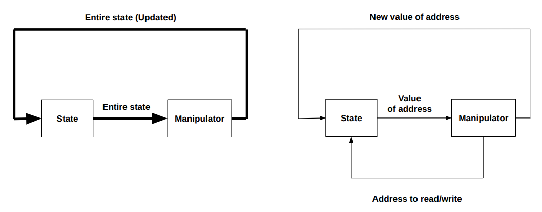
Yes, what we need is an Addressable Memory.
In this section, we're going to implement a very simple—and admittedly foolish—way to build an addressable memory. I say "foolish" because the memory in a typical computer is far more complex and efficient than what we're about to construct. But that's fine—the goal here isn't efficiency. It's to understand the core concept and to get creative with the tools we already have.
So, let’s begin by defining what we want to build. We'll assume we're designing an 8-bit computer. This computer will have a CPU capable of handling 8-bit instructions and an addressable memory (RAM) with an 8-bit address space. That means it will contain \(2^8 = 256\) memory cells, and each cell will store 8 bits of data. A 256-byte random-access memory, which is embarrassingly small by today's standards!
In this section, we’ll focus specifically on building the RAM component.
Given these specifications, our RAM will need:
- 8 address input wires — to specify the memory cell we want to read from or write to.
- 1 read/write control wire — to determine whether the operation is a read or a write.
- 8 data input wires — used only in write mode, to supply the value to store at the specified address.
- 8 data output wires — used only in read mode, to output the value stored at the specified address.
That gives us a total of 17 input wires (8 for address, 8 for data-in, 1 for read/write control) and 8 output wires (for data-out).
Now the challenging question is how to allow only a single 8-bit memory-cell to be read/written, given an address? Not too hard, let's solve the problem for read and write operations independently.
Selective writing
Let's assume that the 8-bit input pins of all the memory cells within our memory are connected to the 8 input pins of the memory component. This would cause the internal value of every memory cell to be updated to the given input value on the next clock cycle. We definitely don't want that! So how can we prevent it?
Remember how a register only stores the inputs values within itself only when a full clock cycle occurs? We can use a similar idea here. Specifically, we need to prevent the clock signal from reaching all memory cells except the one whose address matches the input address. Additionally, when the memory is in read mode, the clock signal should be completely disabled for all memory cells.
Technically, the clock signal should only reach a memory cell if: (addr == cell_index) && write_mode. To achieve this, simply set the input clock signal of each memory cell to: (addr == cell_index) && write_mode && clk
If you're still unsure why this works, try analyzing the value of the equation for different input scenarios.
If write_mode is false, the entire expression evaluates to false for all memory cells, which is exactly what we want—no writes occur. If the address provided to the memory component doesn't match a given cell's index, the expression again evaluates to false, regardless of whether write_mode is true or whether the clock signal is high. This, too, is the intended behavior.
However, when the memory is in write mode and the address matches a specific memory cell’s index, the condition becomes: true && true && clk = clk
This means the global clock signal is effectively passed through to only that memory cell, allowing it to store the input value on the next rising edge—just as intended.
Implementation-wise, we already have AND gates, and the only missing piece is the ability to check the equality of two 8-bit values. As always, it's best to start simple: we'll first design a circuit that can check the equality of two single bits, and then extend that solution to handle multi-bit inputs.
To achieve this, we'll create two modules:
Equals: This module checks the equality of two single bits. Functionally, it's justNot(Xor(a, b)).MultiEquals: This module checks the equality of two multi-bit values. It will be especially useful for comparing memory addresses and decoding instructions in the sections to come.
def Equals(circuit, in_a, in_b, out_eq):
    xor_out = circuit.new_wire()
    Xor(circuit, in_a, in_b, xor_out)
    Not(circuit, xor_out, out_eq)


def MultiEquals(circuit, in_a, in_b, out_eq):
    if len(in_a) != len(in_b):
        raise Exception("Expected equal num of wires!")

    count = len(in_a)
    xor_outs = []
    for i in range(count):
        xor_out = circuit.new_wire()
        Xor(circuit, in_a[i], in_b[i], xor_out)
        xor_outs.append(xor_out)

    inter = circuit.new_wire()
    Or(circuit, xor_outs[0], xor_outs[1], inter)
    for i in range(2, count):
        next_inter = circuit.new_wire()
        Or(circuit, inter, xor_outs[i], next_inter)
        inter = next_inter
    Not(circuit, inter, out_eq)
To keep our implementation of MultiEquals efficient—especially since we'll use many of them in our RAM module—we'll avoid the naive approach of using an array of Equals components followed by a big AND gate.
Instead, we'll take a more optimized route:
- XOR each pair of corresponding bits from the two inputs. This will produce a 1 for any position where the bits differ.
- OR all the XOR results together. If any pair of bits is unequal, the result will be 1.
- NOT the final result. This gives us 1 only if all bits are equal—exactly what we want.
This approach reduces the depth of the logic and avoids constructing redundant gates, making it both faster and more resource-efficient.
Selective reading
The read-mode scenario is even simpler. Memory cells continuously output their internal values to their output pins, regardless of the clock signal—so the clock doesn't matter at all in this case. What we do need is a way to select which register's outputs should be routed to the memory component’s output pins, based on the given address.
To handle this, we introduce a new and very useful component: the multiplexer. Before moving on to our final RAM implementation, let’s take a closer look at how a multiplexer works and how it can be implemented.
A vanilla multiplexer is a digital circuit that takes in \(2^n\) input bits—representing the options to choose from—and another \(n\) bits as a selection input, which tells the circuit which option to access. The output is a single bit: the value of the selected input at the specified index.
You can think of a multiplexer as being conceptually similar to accessing a boolean array: output = data[selection], where data is a bit array with \(2^n\) elements and selection is an \(n\)-bit value indicating which array entry to output.
You can start by building a 2-input multiplexer and then use it to construct larger multiplexers. A 2-input multiplexer takes two data bits as available options and a single selection bit. If the selection bit is 0, the first data bit is output. If the selection bit is 1, the second data bit is output.
Here is a truth-table for the multiplexer described:
| data | sel | out |
|---|---|---|
| 00 | 0 | 0 |
| 00 | 1 | 0 |
| 01 | 0 | 0 |
| 01 | 1 | 1 |
| 10 | 0 | 1 |
| 10 | 1 | 0 |
| 11 | 0 | 1 |
| 11 | 1 | 1 |
Which can be easily constructed using basic logic gates:
out = (!data[0] & sel) | (data[1] & sel)
And here is the equivalent Python component:
def Mux1x2(circuit, in_sel, in_options, out):
    wire_select_not = circuit.new_wire()
    and1_out = circuit.new_wire()
    and2_out = circuit.new_wire()
    Not(circuit, in_sel[0], wire_select_not)
    And(circuit, wire_select_not, in_options[0], and1_out)
    And(circuit, in_sel[0], in_options[1], and2_out)
    Or(circuit, and1_out, and2_out, out)
Now given two \(2^n\) input multiplexers you can build a \(2^{n+1}\) multiplexer!
- A \(2^{n+1}\) input multiplexer has \(2^{n+1}=2 \times 2^n\) inputs.
- Feed the first \(2^n\) input bits to the first multiplexer and the second \(2^n\) input bits to the second multiplexer.
- Connect the first \(n\) bits of the \(n+1\) selection pins to both multiplexers.
- Now you have two outputs—one from each multiplexer. The final output depends on the last (most significant) selection bit. Use a 2-input multiplexer to select between these two outputs and compute the final result.
We can define a meta-function that generates multiplexer component creators, given the number of input pins and a multiplexer component with one fewer selection bit.
For example, you can build a \(2^5\)-input multiplexer using two \(2^4\)-input multiplexers like this: Mux5x32 = Mux(5, Mux4x16)
Then, we’ll iteratively build a \(2^8=256\) input multiplexer, which is exactly what we need for constructing our 8-bit RAM:
def Mux(bits, sub_mux):
    def f(circuit, in_sel, in_options, out):
        out_mux1 = circuit.new_wire()
        out_mux2 = circuit.new_wire()

        sub_mux(
            circuit,
            in_options[0 : bits - 1],
            in_options[0 : 2 ** (bits - 1)],
            out_mux1,
        )
        sub_mux(
            circuit,
            in_sel[0 : bits - 1],
            in_options[2 ** (bits - 1) : 2**bits],
            out_mux2,
        )
        Mux1x2(circuit, [in_sel[bits - 1]], [out_mux1, out_mux2], out)

    return f


Mux2x4 = Mux(2, Mux1x2)
Mux3x8 = Mux(3, Mux2x4)
Mux4x16 = Mux(4, Mux3x8)
Mux5x32 = Mux(5, Mux4x16)
Mux6x64 = Mux(6, Mux5x32)
Mux7x128 = Mux(7, Mux6x64)
Mux8x256 = Mux(8, Mux7x128)
Now we're fully ready to move forward and implement our RAM design!
Chaotic access
First things first—what do we mean by random-access memory?
Because in RAM, it's very efficient to read or write a value at any address, regardless of its position. The key idea is that accessing a memory cell takes the same amount of time no matter which address is used. RAMs are efficient even your read pattern is random!
Now, compare this to how optical disks or hard drives work. These devices have to keep track of the current read/write head position, and to reach a new location, they must seek—move to the requested position relative to where they are. This makes access efficient only when reading or writing data sequentially, like going forward or backward one byte at a time.
However, real-world programs don't access memory so predictably. Instead, they often jump around, requesting data from widely different memory addresses. Since these access patterns are hard to predict, we call it "random access." And RAM is designed specifically to handle such patterns efficiently.
As discussed in the previous section, the read and write modes of our RAM work independently. For the write-mode functionality, we simply need to initialize 256 8-bit registers using a loop and condition their clock signals.
While tracking their outputs in the wire array reg_outs, we’ll use eight Mux8x256 components to select which register's output pins should be routed to the RAM’s output. Eight multiplexers are required because each of our registers has 8 bits.
class RAM:
    def snapshot(self):
        return [self.regs[i].snapshot() for i in range(256)]

    def __init__(self, circuit, in_clk, in_wr, in_addr, in_data, out_data, initial):
        self.regs = []
        reg_outs = [[circuit.new_wire() for _ in range(8)] for _ in range(256)]

        for i in range(256):
            is_sel = circuit.new_wire()
            MultiEquals(circuit, in_addr, num_to_wires(circuit, i), is_sel)
            is_wr = circuit.new_wire()
            And(circuit, is_sel, in_wr, is_wr)
            is_wr_and_clk = circuit.new_wire()
            And(circuit, is_wr, in_clk, is_wr_and_clk)
            self.regs.append(
                Reg8(circuit, is_wr_and_clk, in_data, reg_outs[i], initial[i])
            )

        for i in range(8):
            Mux8x256(
                circuit, in_addr, [reg_outs[j][i] for j in range(256)], out_data[i]
            )
Soon, you’ll realize that our simulator isn't efficient enough to handle transistor-level simulations of RAM, especially as memory size grows. To keep things practical, it makes sense to cheat a little and provide a secondary, faster implementation of RAM—a primitive component described directly in plain Python code, much like how we handled transistors.
class FastRAM:
    def snapshot(self):
        return self.data

    def __init__(self, circuit, in_clk, in_wr, in_addr, in_data, out_data, initial):
        self.in_clk = in_clk
        self.in_wr = in_wr
        self.in_addr = in_addr
        self.in_data = in_data
        self.out_data = out_data
        self.data = initial
        self.clk_is_up = False
        circuit.add_component(self)

    def update(self):
        clk = self.in_clk.get()
        addr = wires_to_num(self.in_addr)
        data = wires_to_num(self.in_data)
        if clk == ZERO and self.clk_is_up:
            wr = self.in_wr.get()
            if wr == ONE:
                self.data[addr] = data
            self.clk_is_up = False
        elif clk == ONE:
            self.clk_is_up = True

        value = self.data[addr]
        for i in range(8):
            self.out_data[i].put(self, ONE if (value >> i) & 1 else ZERO)

        return False
Alright folks—the "state" storage part of our magical CPU/memory duo is now up and running! Now it’s time to build the state manipulator—the CPU itself—and bring everything together to finalize our design of a computer!
The manipulator
Our definition of a computer in this chapter is a machine that can be programmed—something on which you can deploy arbitrary algorithms. We want this program to be replaceable, meaning we may deploy one program now and later substitute it with another. Therefore, it makes perfect sense that the programs on this computer need to be stored in some form of alterable memory.
Our construction of memory is simply an addressable group of memory cells that can store a certain number of bits. So, the "programs" we're referring to must be representable in a binary format—otherwise, how could they persist in memory that only stores data as bits?
In this section, we will discuss how we can assign meaning to numbers and bit patterns. Essentially, we want to design a very simplistic mapping from 8-bit values to "meanings." These mappings will make up the instruction set of our computer. We'll also design circuits that can fetch those values from memory, interpret them, and execute their intended operations.
Before diving into this book's design and implementation of a processor, there’s an important question we need to address. Computer programs need a place to store and manipulate temporary values—much like using a sheet of paper as a draft when solving a math problem. That’s actually one of the primary reasons computers have memory. But we just said that a "program" itself is also data stored in memory. So, is the memory used by the program for drafting its data the same as the memory where the program itself is stored? Or are these two separate memory spaces?
For modern computers, the answer is yes—both the program and its data reside in the same memory. This concept is often summed up by the phrase: code is data, and data is code. It's one of the most brilliant and fundamental ideas that form the basis of modern computers.
The implications of this design—known as the Von Neumann architecture—are profound. When a computer stores both the program and the data it operates on in the same memory, several important things become possible:
- Since programs are stored as data, they can modify themselves during execution, enabling dynamic behavior!
- A program may generate another program: it just needs to dump some instructions on memory and jump to it!
- Errors like buffer overflows can overwrite program instructions, leading to vulnerabilities and exploits.
An interesting perspective is that the reason you can download a compressed executable file from the internet, decompress it, and run it right away is that the data and the program are in the same place!
To keep our computer implementation simple, we will not follow the Von Neumann architecture. Instead, we will assume that code and data are stored in separate memory components. This has made our lives much easier, mainly because we can now read an instruction, decode it, and execute it all in a single clock cycle. If the program and data were both stored in a single memory component, the CPU would need to perform at least two memory reads to execute an instruction: one to read the instruction itself, and another in case the fetched instruction involves accessing memory. (Our current RAM doesn't allow reading from two different memory locations at the same time.) Moreover, the CPU would also require additional circuitry to determine which "stage" it is in during a cycle: Is it supposed to "read" an instruction, or execute one that it has already read and stored in a temporary buffer? We avoided all of this simply by separating the memories.
Decoder
So, we assume that the program is stored in a separate 256-byte memory, where each byte represents an instruction. Since every slot in the program memory represents a single instruction and contains 8 bits of data, we can theoretically have 2^8=256 different instructions. Let’s assign meanings to some of these values to make practical use of them.
Here, I propose a very simple instruction set (a mapping from 8-bit values to meanings/instructions) that will make it easy for us to build a compiler that translates a programming language called Brainfuck into it. (We will explore the details of that language in future sections.)
This instruction set consists of six instructions:
- FWD: Increases the data-pointer by 1, i.e., moves the data-pointer to the next cell.
- BWD: Decreases the data-pointer by 1, i.e., moves the data-pointer to the previous cell.
- INC: Increases the value of the current data cell by 1.
- DEC: Decreases the value of the current data cell by 1.
- JNZ: Jumps to a given address if the value in the current cell is not zero.
- PRNT: Outputs the value of the
Now, here is my proposed mapping from 8-bit patterns to these instructions:
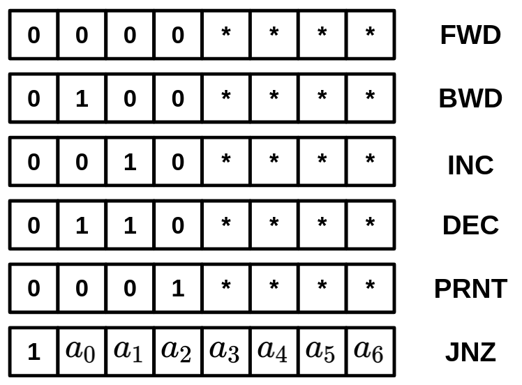 { width=300px }
If you’re wondering why I designed the opcodes of this CPU’s instruction set this way: since we have only six instructions, 3 bits are enough to represent all of them.
However, the JNZ instruction requires an argument: the target address to jump to. One way to pass this argument would be to use the remaining 5 bits of the instruction. But our memory has 256 cells, and 5 bits can only represent 32 locations, leaving 224 locations unreachable, which isn’t ideal.
Instead, a more efficient design is to dedicate the first bit of the 8-bit instruction to indicate whether the instruction is JNZ or something else. If the first bit indicates that it is not JNZ, the CPU can use the remaining bits to determine the exact instruction type.
This approach gives us 7 bits for the jump location, allowing us to access 128 memory locations instead of just 32. This makes much more efficient use of the available space.
Now, while we are okay with this limitation, there are several ways to overcome it. For example, we could make our instructions wider (e.g., 16 bits), or allow some instructions to take extra arguments by performing additional memory reads. For instance, when the current instruction is JNZ, we could wait for another clock cycle and perform an extra memory read to retrieve the memory location to jump to.
However, this would make the JNZ instruction multi-staged, since it would require additional circuitry to read the memory cell following the program counter (PC) in order to obtain the target address in the next clock cycle.
Handling all of that would significantly increase the complexity of our processor. Therefore, to keep things simple, we will assume that jumps cannot target instructions beyond slot #127.
Perfect! Now it's time to get our hands dirty and begin by building hardware that can recognize the type of instruction after fetching it from memory. We'll call this component the Decoder, since it decodes the instruction. The way it works is simple: it performs several equality checks using the MultiEquals component we used earlier when designing the memory.
The Decoder is composed of 5 MultiEquals components to distinguish between FWD, BWD, INC, DEC, and PRNT, as well as a single Equals module responsible for detecting whether the instruction is a JMPs by examining the first bit. The module outputs 6 boolean bits, indicating the type of instruction:
def Decoder(
    circuit,
    in_inst,
    out_is_fwd,
    out_is_bwd,
    out_is_inc,
    out_is_dec,
    out_is_jnz,
    out_is_prnt,
):
    MultiEquals(
        circuit,
        in_inst[0:4],
        [circuit.zero(), circuit.zero(), circuit.zero(), circuit.zero()],
        out_is_fwd,
    )
    MultiEquals(
        circuit,
        in_inst[0:4],
        [circuit.zero(), circuit.one(), circuit.zero(), circuit.zero()],
        out_is_bwd,
    )
    MultiEquals(
        circuit,
        in_inst[0:4],
        [circuit.zero(), circuit.zero(), circuit.one(), circuit.zero()],
        out_is_inc,
    )
    MultiEquals(
        circuit,
        in_inst[0:4],
        [circuit.zero(), circuit.one(), circuit.one(), circuit.zero()],
        out_is_dec,
    )
    MultiEquals(
        circuit,
        in_inst[0:4],
        [circuit.zero(), circuit.zero(), circuit.zero(), circuit.one()],
        out_is_prnt,
    )
    Equals(circuit, in_inst[0], circuit.one(), out_is_jnz)
To get an idea of how this instruction set actually works, let’s look at some examples.
The following program stores the number 2 in the second memory cell and the number 4 in the third memory cell:
0: FWD // Now we are on the second memory-cell
1: INC
2: INC
3: FWD // Moving forward to the third memory-cell
4: INC
5: INC
6: INC
7: INC
Or, this is a program that moves the number from the first memory cell to the second one:
0: INC
1: INC
2: INC

3: DEC
4: FWD
5: INC
6: BWD
7: JNZ(3)
In this program, we assume that the number 3 is stored in the first memory cell by initially incrementing it three times. Then, the move logic follows. In each step, we decrement the value in the first cell and add it to the second cell. This process continues as long as the value in the first cell is not zero (using the JNZ instruction).
(Note: JNZ(3) means setting the program counter register to 3.)
The interesting thing is that you can perform surprisingly complex tasks using such a simple instruction set. If you’re up for a challenge, try implementing a program that calculates the factorial of a number using these instructions.
Fetching the instruction
The computer we are going to implement will be very minimal. In fact, it will have only six different instructions. However, these six instructions are enough to build programs that are more than interesting. Our goal is to design a CPU with enough features to create a Brainfuck compiler that can target its instruction set. We have a whole section dedicated to describing the Brainfuck programming language and the ways you can build complex programs using it. For now, let's focus on the processor's instructions and the way they are fetched.
Before our processor can decode an instruction, it must first fetch it from memory. The first question is: which memory address should be fetched—that is, where is the instruction to be executed located? The next important question is: what is the location of the next instruction that should be fetched and executed?
You might think the next instruction to be executed resides in the program memory cell immediately after the current one. However, that is not always the case. In fact, programs often jump to other parts of the code that are not simply the next instruction. This is how loops and conditional branches are implemented.
To answer the first question, we need a register to hold the current location in program memory from which the instruction should be fetched. Let’s call this register the Program Counter (or simply PC). The PC is initialized to 0, meaning the first instruction to be executed is located at the 0th cell of program memory.
If the current instruction is not a jump, then the next value of the PC should simply be PC + 1. However, if the current instruction is a jump, then the next value of the PC is determined by that instruction. We'll dedicate a module to holding the PC and determining its next value. We’ll call this module the InstructionPointer.
Practically speaking, the InstructionPointer module could first check if a jump is needed (based on the current instruction) and set the instruction pointer to the new value (JNZ_Addr); otherwise, it would simply increment it.
ShouldJump = IsJNZ && (Data[DataPointer] == 0)
InstPtr = ShouldJump ? JNZ_Addr : (InstPtr + 1)
JNZ stands for Jump if Not Zero. It is an instruction that tells the processor to jump to a specific instruction if the value pointed to in data memory is not zero.
Assuming we have a Decoder module that can detect whether the current instruction is JNZ, we can pass the is_jnz flag, along with the data value and the data pointer, to the InstructionPointer module so it can calculate the next value of the program counter.
Here is the implementation of our simplified InstructionPointer module:
def Mux1x2Byte(circuit, in_sel, in_a, in_b, out):
    for i in range(8):
        Mux1x2(
            circuit,
            [in_sel],
            [in_a[i], in_b[i]],
            out[i],
        )


def InstructionPointer(circuit, in_clk, in_is_jnz, in_data, in_addr, out_inst_pointer):
    zero = [circuit.zero()] * 8
    one = [circuit.one()] + [circuit.zero()] * 7

    # should_jump = Data[DataPointer] != 0 && in_is_jnz
    is_data_zero = circuit.new_wire()
    is_data_not_zero = circuit.new_wire()
    should_jump = circuit.new_wire()
    MultiEquals(circuit, in_data, zero, is_data_zero)
    Not(circuit, is_data_zero, is_data_not_zero)
    And(circuit, in_is_jnz, is_data_not_zero, should_jump)

    # InstPointer = should_jump ? in_addr : InstPointer + 1
    inst_pointer_inc = [circuit.new_wire() for _ in range(8)]
    inst_pointer_next = [circuit.new_wire() for _ in range(8)]
    Adder8(
        circuit,
        out_inst_pointer,
        one,
        circuit.zero(),
        inst_pointer_inc,
        circuit.new_wire(),
    )
    Mux1x2Byte(
        circuit,
        should_jump,
        inst_pointer_inc,
        in_addr + [circuit.zero()],
        inst_pointer_next,
    )

    return Reg8(circuit, in_clk, inst_pointer_next, out_inst_pointer, 0)
Next, we introduce an InstructionMemory, which is a 256-byte RAM that stores our program. We connect the program-counter output of the InstructionPointer's outputted PC to the InstructionMemory, which outputs the fetched instruction. This instruction is then passed to a Decoder module again so it can be decoded, determining what action the processor should take next.
def InstructionMemory(circuit, in_clk, in_inst_pointer, out_inst, code):
    return FastRAM(
        circuit,
        in_clk,
        circuit.zero(),
        in_inst_pointer,
        [circuit.zero()] * 8,
        out_inst,
        code,
    )
Remember how we decided to separate the program and its data into different memory modules? That means we need another pointer and memory to manage. Similar to how we introduced the Program Counter to track the current instruction, our processor will also have a register called the Data Pointer. As the name suggests, this register points to a specific cell in the data memory. By default, it is initialized to zero, pointing to the first memory cell.
Unlike the InstructionPointer, which is automatically incremented on every clock tick, the DataPointer usually remains unchanged. Its value is updated only when a FWD or BWD instruction is executed, which increment or decrement the pointer, respectively.
To describe this behavior using multiplexers, we can introduce two input signals, is_fwd and is_bwd, which are provided by the Decoder module and indicate whether the current instruction is FWD or BWD.
From these signals, we can derive an intermediate signal is_fwd_bwd that indicates whether the current instruction modifies the data pointer at all. If neither instruction is active, the data pointer retains its previous value. We can also define a data_pointer_next signal that holds data_pointer + 1 when is_fwd is high, and data_pointer - 1 when is_bwd is high.
IsFwdOrBwd = IsFwd | IsBwd
DataPtrNext = IsFwd ? (DataPtr + 1) : (DataPtr - 1)
DataPtr = IsFwdOrBwd ? DataPtrNext : DataPtr
In the Python implementation of this logic, we first precompute the incremented and decremented versions of the data pointer by adding 0b00000001 and 0b11111111 (i.e., –1 in two’s complement) to the current data pointer, respectively. We then feed either the original value, the incremented value, or the decremented value back into the data pointer register, following the logic described above using two multiplexers.
def DataPointer(circuit, in_clk, in_is_fwd, in_is_bwd, data_pointer):
    one = [circuit.one()] + [circuit.zero()] * 7
    minus_one = [circuit.one()] * 8

    # data_pointer_inc = data_pointer + 1
    data_pointer_inc = [circuit.new_wire() for _ in range(8)]
    Adder8(
        circuit, data_pointer, one, circuit.zero(), data_pointer_inc, circuit.new_wire()
    )

    # data_pointer_inc = data_pointer - 1
    data_pointer_dec = [circuit.new_wire() for _ in range(8)]
    Adder8(
        circuit,
        data_pointer,
        minus_one,
        circuit.zero(),
        data_pointer_dec,
        circuit.new_wire(),
    )

    data_pointer_next = [circuit.new_wire() for _ in range(8)]
    in_is_fwd_bwd = circuit.new_wire()
    Or(circuit, in_is_fwd, in_is_bwd, in_is_fwd_bwd)
    tmp = [circuit.new_wire() for _ in range(8)]
    Mux1x2Byte(circuit, in_is_bwd, data_pointer_inc, data_pointer_dec, tmp)
    Mux1x2Byte(circuit, in_is_fwd_bwd, data_pointer, tmp, data_pointer_next)

    return Reg8(circuit, in_clk, data_pointer_next, data_pointer, 0)
The data-pointer register points to a memory location, right? That means we also need a DataMemory module to actually store data. This module takes the data address to be read from or written to as an input (which is driven by the data pointer). It also receives two control wires, is_inc and is_dec, which indicate whether the processor has reached an INC or DEC instruction and should increment or decrement the value stored at the given memory location on the next clock cycle. The module outputs the current value stored in the memory slot being pointed to.
Our DataMemory module is essentially a wrapper around a RAM module. The RAM module’s write-enable flag is set to true only when either is_inc or is_dec is high. The new value to be written to memory is selected using a multiplexer between two precomputed values: data_inc and data_dec.
def DataMemory(circuit, in_clk, in_addr, in_is_inc, in_is_dec, out_data):
    one = [circuit.one()] + [circuit.zero()] * 7
    min_one = [circuit.one()] * 8

    is_wr = circuit.new_wire()
    Or(circuit, in_is_inc, in_is_dec, is_wr)

    data_inc = [circuit.new_wire() for _ in range(8)]
    data_dec = [circuit.new_wire() for _ in range(8)]
    Adder8(circuit, out_data, one, circuit.zero(), data_inc, circuit.new_wire())
    Adder8(circuit, out_data, min_one, circuit.zero(), data_dec, circuit.new_wire())
    data_next = [circuit.new_wire() for _ in range(8)]
    Mux1x2Byte(circuit, in_is_dec, data_inc, data_dec, data_next)

    return FastRAM(
        circuit, in_clk, is_wr, in_addr, data_next, out_data, [0 for _ in range(256)]
    )
Finally, our computing machine begins operating when all of these modules are brought together and properly connected. We also provide a snapshot() function, which allows us to inspect the internal state of the machine for debugging purposes:
class CPU:
    def snapshot(self):
        print("Data Pointer:", self.data_pointer.snapshot())
        print("Instruction Pointer:", self.inst_pointer.snapshot())
        print("RAM:", self.ram.snapshot())

    def __init__(
        self,
        circuit: Circuit,
        in_clk: Wire,
        code: str,
        out_ready: Wire,
        out_data,
    ):
        inst_pointer = [circuit.new_wire() for _ in range(8)]
        inst = [circuit.new_wire() for _ in range(8)]

        data_pointer = [circuit.new_wire() for _ in range(8)]
        data = [circuit.new_wire() for _ in range(8)]

        is_fwd = circuit.new_wire()
        is_bwd = circuit.new_wire()
        is_inc = circuit.new_wire()
        is_dec = circuit.new_wire()
        is_jmp = circuit.new_wire()
        is_prnt = circuit.new_wire()

        Forward(circuit, is_prnt, out_ready)
        for i in range(8):
            Forward(circuit, data[i], out_data[i])

        # inst = Inst[inst_pointer]
        self.rom = InstructionMemory(circuit, in_clk, inst_pointer, inst, code)

        # is_fwd = inst[0:4] == 0000
        # is_bwd = inst[0:4] == 0100
        # is_inc = inst[0:4] == 0010
        # is_dec = inst[0:4] == 0110
        # is_prnt = inst[0:4] == 0001
        # is_jmp = inst[0] == 1
        Decoder(circuit, inst, is_fwd, is_bwd, is_inc, is_dec, is_jmp, is_prnt)

        # inst_pointer =
        #   if is_jmp: inst[1:8]
        #   else: inst_pointer + 1
        self.inst_pointer = InstructionPointer(
            circuit, in_clk, is_jmp, data, inst[1:8], inst_pointer
        )

        # data_pointer =
        #   if is_fwd: data_pointer + 1
        #   if is_bwd: data_pointer - 1
        #   else: P
        self.data_pointer = DataPointer(circuit, in_clk, is_fwd, is_bwd, data_pointer)

        # data = Data[data_pointer]
        #   if is_inc: Data[data_pointer] + 1
        #   if is_dec: Data[data_pointer] - 1
        #   else: Data[data_pointer]
        self.ram = DataMemory(circuit, in_clk, data_pointer, is_inc, is_dec, data)
Remember the PRNT instruction? It allows our computer to communicate with the external world! Our interface consists of two outputs from the CPU module: out_data and out_ready.
out_datais an 8-bit output representing the value the CPU intends to send to the outside world (for example, it could be the letterHin a program that printsHello world!).out_readyis a 1-bit flag indicating whether there is valid data on out_data to be written.
To satisfy this interface, we simply connect the is_prnt output from our Decoder to out_ready and forward the output of the DataMemory module to out_data. This way, out_data always reflects the value at the current data pointer location, but it is only recognized as an output when the CPU is executing a PRNT instruction, just as intended!
Now, let’s write a compiler/assembler that can convert Brainfuck code into opcodes runnable by our processor! (Don’t worry, we’ll dive deeper into that language later. For now, we just need to feed some real code into our computer to see if it actually works!)
def compile(bf):
    opcodes = []
    locs = []

    for c in bf:
        if c == ">":
            opcodes.append(0)  # FWD 00000000
        elif c == "<":
            opcodes.append(2)  # BWD 00000010
        elif c == "+":
            opcodes.append(4)  # INC 00000100
        elif c == "-":
            opcodes.append(6)  # DEC 00000110
        elif c == ".":
            opcodes.append(8)  # PRNT 00001000
        elif c == "[":
            locs.append(len(opcodes))  # Do nothing!
        elif c == "]":
            opcodes.append(1 + (locs.pop() << 1)) # JNZ [7-BIT LOCATION]0

    return opcodes + [0 for _ in range(256 - len(opcodes))]
Here, I have a working Brainfuck program that prints the Fibonacci sequence. Simply load it into the program memory and let it run. If the outputs are correct, then all parts of your computer are functioning perfectly.
Notice that in each clock cycle, we check whether the out_ready flag is set to 1. Whenever this happens, the value in the out_data signal is printed. This allows the CPU to communicate with the external world!
if __name__ == "__main__":
    circ = Circuit()
    clk = circ.new_wire()

    out_ready = circ.new_wire()
    out = [circ.new_wire() for _ in range(8)]

    OSCILLATOR = "OSCILLATOR"

    clk.put(OSCILLATOR, ZERO)

    code = "+>+[.[->+>+<<]>[-<+>]<<[->>+>+<<<]>>[-<<+>>]>[-<+>]<]"

    cpu = CPU(circ, clk, code, out_ready, out)
    print("Num components:", circ.num_components())

    while True:
        circ.stabilize()

        if out_ready.get() and clk.get():
            print(wires_to_num(out))

        clk.put(OSCILLATOR, 1 - clk.get())
Unfortunately, the CPU we just implemented is not a 100% accurate implementation of Brainfuck, the slight difference is that in standard Brainfuck, the operation [ acts like a JZ (Jump if zero!) instruction, it jumps to the corresponding ] when the data in the data-pointer is zero. In our implementation, the [ operator is compiled to nothing, and is ignored, although this doesn't stop us for having loops!
What about keyboards, monitors and etc?
Our processor’s connection with the external world is currently very limited. Although we have enabled it to “print” values to a console, there is much more work needed to make it resemble a real computer with a monitor, keyboard, mouse, and so on.
Even though this may seem complicated, the general idea remains the same: you need to allow your CPU to expose some of its internal state and provide flags that indicate when outputs are available for external modules (like a console, or even a full-featured monitor capable of displaying images using a grid of RGB values). Then, all you have to do is design third-party hardware that understands these outputs and interprets them correctly.
A potentially more efficient way to render a computer screen (e.g., the desktop of an operating system) is to store RGB values directly in RAM and share a portion of that RAM with another hardware module that mirrors the values on a display.
So far, we have discussed how your processor can output values. But what about reading input from the external world, like a key press on a keyboard or mouse movement? The principle is the same. A third-party hardware module can provide two signals, out_ready and out_data. For a keyboard, out_ready indicates whether a key has been pressed, and out_data holds the ASCII value of the pressed key. These signals can be connected to in_ready and in_data on your processor, giving it access to external input.
The original Brainfuck language has an instruction for reading an 8-bit input from the user into the current data cell. Let’s assume a new instruction INP for similar functionality (in Brainfuck, this is represented by ,). While we haven’t implemented it here, you can try it as an exercise:
- When the processor reaches an
INPinstruction, it should pause incrementing the PC. - It should wait for
in_readyto become true. - Once ready, it should capture the value from
in_dataand store it in the current data-pointer location.
This approach allows your CPU to both read from and write to the external world, completing the basic model of a working computer.
When you hate wires
A computer screen/monitor is effectively a grid of pixels, which their color is determined by a computer through a hardware interface. Your screen may have millions of pixels, but if you look at the port by which your screen is connected to your computer, you may only see a few wires. This means something important: the pixel data are fed to your monitor "serially". Whenever a new frame to be shown on your screen is ready, your computer will start transferring each pixel through that port to your monitor, which is effectively a whole computer on its own that can understand the raw pixel data transferred to it and set the color of each pixel under its control according to it.
Now, look closer, logically speaking each pixel on your screen should have been somehow be connected to the screen's main board in order to be controlled, but you won't see that many wires connected to your pixel-array either. So what's happening here? How is the value of each individual pixel set, if there isn't an independent wires for each pixel? The answer lies in a simple trick we use in everyday life too: e.g when you try to distribute question sheets in a classroom during a test. You don't need to go to every student and give him his sheet one-by-one, it's inefficient. You'll just give the student in the front a group of sheets and they will just pick one and pass the rest to the student behind them. Each pixel is in practice also a register that stores the RGB components of the pixels, and the pixels are all conneced to each other. When you feed the very first pixel a value, it will store that value in itself, and spit out the old value to the next pixel. These values will all get shifted in a domino-like effect. Now, if you have 2000-pixels and feed the very first pixel 2000 values in each clock cycle (Yes, your processor is not the only component that has a clock signal), you can effectively set all of these pixels your desired values, and you won't need 2000 wires, since your only endpoint to input the pixel values will be the first pixel. The values for last pixel is fed first and the value for the first pixel is fed last! The registers that are chained together with such a structure are called shift registers, and this is in fact a very useful design pattern seen in a lot of hardware.
Poking your processor
I know, I know. Although our basic computer model can compute correctly and handle input and output, it still leaves many questions unanswered. Perhaps the most important question right now is this: imagine my computer is busy running a computationally heavy algorithm. It doesn’t have an INP instruction anywhere in its code, but it still wants to detect if the user pressed a key on the keyboard and respond accordingly.
For example, what if the intended behavior is to cancel the running algorithm and jump to another routine when a key is pressed? This is where one of the most important solutions in modern computers comes into play: interrupts.
Interrupts, as the name suggests, allow us to temporarily take control and provide external inputs to a processor mid-execution. They literally “interrupt” the current execution flow so that the processor can execute a different routine in response to some event—like a key press on a keyboard or an incoming network packet.
Interrupts are essential in modern computers because constantly checking for new inputs would be inefficient. Instead, it’s better for external events to notify the processor when attention is needed. The concept is actually quite simple:
Imagine we have an input signal in_interrupt for our processor, which is a boolean flag indicating that an interrupt has occurred. This flag can represent any external event, not just a key press, signaling that the current execution flow should be paused so the processor can handle the input.
Before executing the currently fetched instruction, the processor can check the value of this flag. If it is true, the processor updates the program counter to point to a special location in program memory. That location contains an interrupt handler routine, which defines how the processor should respond to the event—for example, storing the pressed key in a memory buffer.
Once the interrupt handler has finished executing, the processor must resume its previous execution. Otherwise, the original program flow would be lost. The solution is simple: store the current PC before jumping to the interrupt handler, and restore it after the handler finishes. This ensures that the processor can continue exactly where it left off.
The most genious interrupt ever
By now, everything about a computer should make sense to you. You can probably imagine how a system as complex as a server responding to a web request and a browser rendering its response can ultimately be described using nothing more than transistors!
But there’s still one big question that isn’t immediately obvious: how can a processor execute two different processes at the same time?
The answer may surprise you: the interrupt system is enough to implement multitasking! You just need a special kind of interrupt that triggers your CPU at fixed intervals: a timer interrupt, for example, that fires every 10 milliseconds.
How does this help? Remember that when an interrupt occurs, the processor stops executing the current process and jumps to a special part of memory where the interrupt handler resides. What if the interrupt handler decides to switch to another process instead of returning to the previous one? That’s exactly the idea behind an operating system: to determine what the next value of the program counter should be!
Interesting, right? I’ll stop here, I’m confident you now have the tools to figure out the rest!
Important questions you should ask yourself
What is the first program that runs on my computer?
We saw that cpus are simple devices that can fetch instructions from memory, run them and write the side effects back to the memory. So, what are the first instructions that are being run in a computer? When you turn your computer on, your RAM is empty, and there are no instructions, so how does it start to load anything when a RAM is absolutely empty on a startup?
The answer is: although your computer has an empty ram, we can still trick your computer, making it believe that some constant pieces of data do exist in the very first bytes of your RAM, and put some initial programs there.
How can programs not conflict with each other in memory locations?
This is a question that you might not have asked yourself but is an important one: when you compile a program, you will get a raw binary that contains the cpu opcodes that need to be executed. Those opcodes that have something to do with your RAM, may use static locations in your memory. Now, imagine you want your computer to load and maintain multiple programs on your ram at the same time. Since the programs are using static locations, there is a very high probability that they will use the same locations of memory for storing data. How does a cpu prevent that? Sometimes this could be malicious too, a program may try to read/write locations on memory that are not for itself (E.g a malicious program may try to read the password you entered for logging in to your shell program)
If you are nerd enough to write an OS yourself
You can’t really understand the way a modern computer’s cpu work without writing an operating system for it. Unfortunately, writing an operating system for a popular CPU like x86-64 involves a lot of details that are not necessarily helpful for a book like this. I’ll try my best to explain most of the important questions you might have here, but I highly encourage you to write a simple OS yourself! Here is a good roadmap for an OS project:
- Read about cross-compiler and try to build a C compiler targeting raw binaries on your CPU
- Write a bootloader that is able to print something on the screen
Brainfuck
Most people say it’s crucial to learn C if you want to be a good programmer. I say you only become truly skilled in programming when you learn how to program in a strange programming language named Brainfuck. Brainfuck is a language where you can only build working programs if you have a solid engineering mindset. Created in 1993 by Urban Müller, Brainfuck is an esoteric programming language: designed mainly for fun and as a challenge. Learning to program in Brainfuck is a great way to see and understand how amazing things can be built by combining really simple components.
Brainfuck is extremely minimalistic, consisting of only eight simple commands. It’s easy to learn but hard to build anything meaningful with! Despite its simplicity, it can be mathematically proven that Brainfuck is Turing-complete, which means you can theoretically build web browsers, 3D games, and all kinds of complex software with it.
The processor we are going to design and implement in this chapter will be heavily inspired by this language. In fact, the CPU will have instructions almost identical to those in Brainfuck (with some slight differences). Therefore, it’s crucial to first take a quick look at the language and see how different programs can be built with it. After that, we will explore how to build hardware capable of understanding and executing Brainfuck programs.
Brainfuck is a minimalistic language that works with a simple array of memory cells, each initially set to zero, and a pointer that moves along these cells. You can increase or decrease the value in the current cell, move the pointer to adjacent cells, and perform input and output operations based on the value at the pointer’s position. The language also lets you jump to other parts of your code depending on whether the value of the current cell is zero or not. This basic setup enables surprisingly powerful computation through careful manipulation of memory and control structures.
Here is the specification of the instructions:
| Instruction | Description |
|---|---|
| > | Increment the data pointer |
| < | Decrement the data pointer |
| + | Increment the byte at the data pointer |
| - | Decrement the byte at the data pointer |
| . | Output the byte at the data pointer |
| , | Store an input at the data pointer |
| [ | If the byte at the data pointer is zero, jump forward to the command after the corresponding ] |
| ] | If the byte at the data pointer is not zero, jump back to the command after the corresponding [ |
Nothing explains the language better than a few examples:
Storing a value in a memory cell
Setting the value of different slots is quite easy. You just have to navigate to the target cell using the <> instructions, and then repeat + as many times as needed. For example, the following code sets the first memory cell to 5 and the second memory cell to 7:
+++++       (set cell #0 to 5)
> +++++++   (move to cell #1 and set it to 7)
Moving a value from one cell to another
The values you'll be working with in your program are not always static. Sometimes, you'll want to move an existing value from one memory cell to another. That's where the loop instructions [] come in handy. The code below simply decrements the source cell and increments the target cell as long as the source cell is above zero, effectively zeroing out the source cell and incrementing the target cell by the same amount:
+++         (set cell #0 to 3)
[->+<]      (move the value from cell #0 to cell #1)
Copying a value from one cell to another
The fact that the move operation will wipe out the source cell is sometimes inconvenient. What if you want to copy a value while preserving the original value of the source cell? This is typically done by decrementing the source cell while incrementing both the target cell and a temporary memory cell. You then move the value from the temporary cell back into the source cell, restoring its original value. The code would look like this (we are copying cell #0 to cell #1, using cell #2 as temporary storage):
+++         (set cell #0 to 3)
[->+>+<<]   (move the value in cell #0 to both cell #1 and #2)
>> [-<+>]   (restore the value of cell #0 by moving the value in cell #2 to back cell #0)
Adding two cells together
Now, an important point when moving or copying values is that the target cell is not necessarily zero. In this case, you are effectively adding two numbers together. (Voila! The first useful case of Brainfuck!):
+++         (set cell #0 to 3)
> ++++ <    (set cell #1 to 4 and go back to cell #0)
[->+<]      (move the value from cell #0 to cell #1)
Zeroing out a cell
So, what if you want to ignore the current value of the target cell and ensure it holds exactly the value from the source cell? Easy! Just clear out the target cell before performing the move. Clearing a cell is as simple as using a loop with a decrement instruction: [-]
+++         (set cell #0 to 3)
> ++++ <    (assume the target cell is not zero)
> [-] <     (clear out the target cell)
[->+<]      (perform the move operation)
These are some very simple and primitive operations you can perform in a Brainfuck program. Things get more interesting when you start nesting loops, for example, you can implement multiplication by placing one loop inside another. We'll take a much deeper approach to implementing Brainfuck programs in the later sections.
Now that you're convinced real programs can be implemented using Brainfuck, I have good news for you: Brainfuck's specification is almost identical to the instruction set we designed for our processor in the previous sections! In fact, you can directly translate each character in a Brainfuck program into an instruction for our processor. We even wrote a simple compiler that does exactly this in the previous sections!
A playground
I would like us to dig deeper into Brainfuck, but it's a bit hard to try running and debugging these programs on our simulated hardware. So, let's set that processor aside and instead learn this wonderful language using an interpreter or compiler that runs on your own computer. We'll start by writing an interpreter for the language.
The original Brainfuck machine specification has 30,000 memory cells, each storing an 8-bit byte (an unsigned integer between 0 and 255). First, we will initialize an array of that size. Then we'll write a while loop that increments the program counter and jumps back whenever it reaches a [ or a ] instruction (remember the JNZ instruction we had on our processor?).
To determine which ] instruction corresponds to which [, we'll maintain a stack.
The following code is a Brainfuck interpreter written in Python, which executes a "Hello World!" program written in Brainfuck.
code = '''
++++++++[>++++[>++>+++>+++>+<<<<-]>+>+>->>+[<]<-]>>.>
---.+++++++..+++.>>.<-.<.+++.------.--------.>>+.>++.
'''

memory = [0] * 30000
ptr = 0
pc = 0

stack = []
while pc < len(code):
    if code[pc] == ">":
        ptr = (ptr + 1) % 30000
    elif code[pc] == "<":
        ptr = (ptr - 1) % 30000
    elif code[pc] == "+":
        memory[ptr] = (memory[ptr] + 1) % 256
    elif code[pc] == "-":
        memory[ptr] = (memory[ptr] - 1) % 256
    elif code[pc] == "[":
        stack.append(pc)
    elif code[pc] == "]":
        top = stack.pop()
        if memory[ptr] != 0:
            pc = top
            continue
    elif code[pc] == ".":
        print(chr(memory[ptr]), end="")

    pc += 1
If you want to achieve maximum speed when running a Brainfuck program, it’s worth noting that Brainfuck can be directly transpiled to C. You only need to initialize a few variables and then perform the following substitutions:
unsigned char mem[30000] = {0};
unsigned int pc = 0;
| Instruction | Equivalent C code |
|---|---|
| > | ptr++; |
| < | ptr--; |
| + | mem[ptr]++; |
| - | mem[ptr]--; |
| . | putchar(mem[ptr)); |
| , | mem[ptr] = getchar(); |
| [ | while(mem[ptr] != 0) { |
| ] | } |
Here is a Brainfuck-to-C transpiler written in Python (bf2c.py):
print('#include <stdio.h>')
print('void main() {')
print('unsigned char mem[30000] = {0};')
print('unsigned int ptr = 0;')

mapping = {
    '>': 'ptr++;',
    '<': 'ptr--;',
    '+': 'mem[ptr]++;',
    '-': 'mem[ptr]--;',
    '[': 'while(mem[ptr]) {',
    ']': '}',
    '.': 'putchar(mem[ptr]);',
    ',': 'mem[ptr] = getchar();'
}

bf = input()

for ch in bf:
    if ch in mapping:
        print(mapping[ch])

print('}')
To use this tool for running your Brainfuck programs:
- Write your Brainfuck program in a file called
main.bf. - Transpile it to C:
python3 bf2c.py < main.bf > main.c - Compile the C program:
gcc main.c - Run the program:
./a.out
Now let's try building some things with this language!
Hello Brainfuck!
Printing a string is one of the first things people do when learning a new programming language. Surprisingly, printing text isn't that straightforward in an esoteric language like Brainfuck. Since a Brainfuck program's inputs and outputs are bytes, we need to work with an 8-bit character encoding (such as ASCII) in order to handle strings.
The instruction . is responsible for outputting bytes, and it prints the byte stored in the memory cell that the program is currently pointing to. Therefore, we somehow need to place the desired ASCII value in that memory cell before printing it.
A naïve approach would require many + instructions to increment the current memory cell until it reaches the ASCII value of the desired character. For example, we would need 72 + instructions to print the character H.
However, there are ways to optimize this process. Once the value 72 is already in memory, we don't need to add 69 + instructions in another memory cell to print the next letter, E. Instead, we can simply subtract 3 from the current value (since 72-3=69) and print again.
Using this idea, we can write a Brainfuck program that prints "HELLO WORLD" in roughly 160 instructions:
+++++++++++++++++++++++++++++++++++
+++++++++++++++++++++++++++++++++++
++.---.+++++++..+++.                ; Print 'HELLO'

>++++++++++++++++++++++++++++++++.< ; Print ' '

++++++++.--------.+++.------.------
--.                                 ; Print 'WORLD'
Printing the space character (ASCII code 32) required a large jump in value, so we chose to generate it in a separate memory cell. To do this, we moved the cursor to the next cell, incremented it 32 times, printed it, and then moved the cursor back to its original position.
From now on, instead of jumping to different memory locations using the <> instructions directly, we will improve readability by assigning names to memory locations. When we want to move to a different memory cell, we will simply refer to it by its name.
For example, imagine that we have named the memory cells of our machine like this:
0 1 2 3 4 5 6 7 8 9 ...
    A     B   C
Imagine we want to add the values in memory locations B and C to A. Assuming we are currently at the 0th memory cell, we can write the code like this:
>>>>>[-<<<+>>>]>>[-<<<<<+>>>>>]
As humans, it would be very difficult to analyze what is happening in this code. We can make it significantly more readable by expressing it like this:
B[-A+B]C[-A+C]
Look how easier it gets when you describe Brainfuck algorithm using this representation:
Moving from A to B: A[-B+A]
Copying from A to B: A[-B+T+A]T[-A+T]A
We can actually write a compiler that handles all these names and memory management for us, making our lives much easier!
Befriending complexity
As you write more complicated programs in Brainfuck, you will soon notice that the immense amount of complexity becomes unmaintainable over time, and eventually you won’t be able to add more logic or features to your programs. That’s when you start missing functions, classes, and other tools that your favorite high-level programming language normally provides for free.
Brainfuck is very similar to the assembly language of a very simple CPU. Because of that, it makes sense to start describing our programs in a higher-level language that can later be translated into Brainfuck. This makes it much easier to build complex programs that can run on our CPU without losing our sanity.
I have decided not to guide you through the full process of building a compiler, because that topic is a world of its own. Compilers are programs that convert strings in one language into strings in another language. In essence, they are string manipulation programs. Even if you don’t know the inner workings of a modern compiler, you probably already have some intuition about how one works. For that reason, we won’t go deep into compiler construction in this book. The main goal here is to understand the core ideas, not to build production-level implementations!
Instead of designing a completely new language that compiles to Brainfuck, a simpler approach is to write a Python library that generates Brainfuck code. This library will allow us to split our Brainfuck applications into modules, making them much easier to manage.
In this framework, the modules of our Brainfuck application will live inside Python functions. Each function will accept a BrainfuckGenerator class as its first argument, while the other inputs and outputs of the module will be memory locations (Pointers).
The generator class will provide an append method, allowing modules to emit raw Brainfuck code into the generator. In addition, it would be useful for the generator class to include memory management functionality, enabling users to allocate and free memory cells when needed. This way, users won’t have to worry about accidentally using memory cells that are already in use by other modules, and can instead focus on the application’s logic.
Here is an example of what this might look like:
class Pointer:
    def __init__(self, pos: int):
        self.pos = pos


class BrainfuckGenerator:
    def __init__(self):
        self.code = ""
        self.pos = 0
        self.allocated = set()

    def append(self, code):
        self.code += code

    def alloc(self) -> Pointer:
        pos = self.pos + 1
        while pos in self.allocated:
            pos += 1
        self.allocated.add(pos)
        return Pointer(pos)

    def free(self, ptr: Pointer):
        self.allocated.remove(ptr.pos)

    def move(self, target: Pointer):
        if target.pos > self.pos:
            self.code += ">" * (target.pos - self.pos)
        else:
            self.code += "<" * (self.pos - target.pos)
        self.pos = target.pos
Our Brainfuck code generator helps us keep track of the memory locations used by different modules in our Brainfuck programs and prevents conflicts. The generator does not allow you to move to different memory locations manually; instead, you must use the move function. This function keeps track of the current location of the data pointer and generates the necessary < or > instructions whenever the pointer needs to move.
The alloc function finds the first unused memory location and marks it as allocated. The free function allows the user to release a memory cell again by removing its flag from the self.allocated set.
Great! Now let's implement some modules. We'll start with simple ones: a module that zeroes out a memory cell by moving to it and decrementing it until it reaches 0 (zeroize), and a module for placing a fixed number into a memory cell (fill). The fill module will make use of the zeroize module.
def zeroize(bf: BrainfuckGenerator, target: Pointer):
    bf.move(target)
    bf.append('[-]')


def fill(bf: BrainfuckGenerator, target: Pointer, val: int):
    zeroize(bf, target)
    bf.move(target)
    bf.append('+' * val)
A more complicated example is the copy operation. As you know, we need a third memory cell in order to copy a value from a source cell to a destination cell. We will use the alloc function to find an unused cell, and once we are finished with it, we will free it so that other modules can use it later.
def copy(bf: BrainfuckGenerator, src: Pointer, dst: Pointer):
    tmp = bf.alloc()

    # Move src to tmp and dst
    bf.move(src)
    bf.append("[-")
    bf.move(tmp)
    bf.append("+")
    bf.move(dst)
    bf.append("+")
    bf.move(src)
    bf.append("]")

    # Move tmp to src
    bf.move(tmp)
    bf.append("[-")
    bf.move(src)
    bf.append("+")
    bf.move(tmp)
    bf.append("]")

    bf.free(tmp)


bf = BrainfuckGenerator()
copy(bf, Pointer(5), Pointer(8))
print(bf.code)
We can even take advantage of Python’s with expressions to implement for loops:
class For:
    def __init__(self, bf: BrainfuckGenerator, i: Pointer, count: Pointer):
        self.bf = bf
        self.i = i
        self.count = count

    def __enter__(self):
        copy(self.bf, self.count, self.i)
        self.bf.move(self.i)
        self.bf.append('[')

    def __exit__(self, exc_type, exc_val, exc_tb):
        self.bf.move(self.i)
        self.bf.append('-]')
Here is a program that prints the letter A five times:
bf = BrainfuckGenerator()

i = bf.alloc()
cnt = bf.alloc()
ascii_a = bf.alloc()

fill(bf, ascii_a, 65)
fill(bf, cnt, 5)
with For(bf, i, cnt):
    bf.move(ascii_a)
    bf.append('.')
See how easy it is getting? The more you organize stuff into modules and the more abstractions you make, the easier it gets to describe any kind of logic in a weird, unimaginably hard to maintain language like Brainfuck.
An art project
I have always dreamed of writing something extraordinarily complicated using the Brainfuck language. When a computer scientist says, you can absolutely do any type of computation using Brainfuck, it really means something, but you won't believe it unless you see it in action. That's why I was thinking of writing something as complicated as a 3D renderer using this language, and call it an art project. Because, it really is art! Just imagine how a bunch of <>[]+- characters can, in theory, be used to generate a photo-realistic render of a 3D scene! And if we do this, we can claim the stupidly simple processor we created in previous sections is in fact able to run something like a 3D game too!
I did really start writing a ray-tracer for this language, named it BFRT (Brainfuck Ray Tracer) but never finished it. It is extremely difficult to be honest, specially if you lose passion along the way, but indeed possible. But maybe you are more brave than me and can finish what I started, and if you really do it, your work is truly a masterpiece that will amaze a lot of programmers! If you don't have any idea what a ray-tracer is and how it works, don't worry, we'll discuss it in chapter 3. But don't forget to get back to this section and give a second thought on trying this challenge!
Here are some of my findings in this journey:
- You are not alone, a lot of people have tried implementing complicated stuff using Brainfuck. Some of those insane people have even created an algorithm library for this language, so that you don't have to think about things like how to calculate equality of two memory cells as a boolean, or how to implement something like an if block, and prevent you from reinventing the wheel. Just search for "Brainfuck algorithms" and you'll find those!
- You might wonder, well, you'll at least need floating-point operations to be able to do something like 3D rendering and since Brainfuck only gives you increment/decrementing of values up to 255, this is just impossible. And yes, that actually is the most challenging part of the project. It looks impossible but hey, aren't all these "floating-point" stuff also made of a bunch of simple AND/OR/NOT operations? And I can show you how those operations look like in that langauge. So what prevents you to implement your own IEEE 754 floating-point module in Brainfuck? Floating point numbers are stored as bytes in the end. A float32 number can be stored in 4 memory-cells of the Brainfuck environment. And just like how things like adding/multiplying/dividing floating-point numbers using bare transistors, it is indeed possible to describe them using Brainfuck programs too. In the end though, I decided not to implement IEEE-754 and instead represent floating point numbers as decimals (Integers under the hood, but with an imaginary dot in the middle of the number) This way, floating-point additions will be no different than integer additions, and floating-point multiplication is nothing but the regular integer multiplication, shifted to right to lose some of the digits from the right side. (E.g, imagine we want to multiply 12.34 by 56.78. We would simply calculate 1234*5678, and then put dot before the last 4 digits (700.6652), and ignore the last 2 floating point digits, 700.66). The division operation would has a different story.
- In order to implement floating-point division, look for algorithms that will allow you to calculate floating-point reciprocals. This way, division will become a multiplication: a/b=a*(1/b)
- After having floating-point basic operations, the only remaining math operation that you will need in order to render a simple scene is the square-root calculation for floating point numbers.
- Try writing "unit-test"s for each operation you'll implement. Since brainfuck programs are massive junks of random-looking characters, it becomes very important to handle complexitiy and keep your system maintainable. Specially, make sure your floating-point operations all work as expected.
Now even if you successfully implement a working ray-tracer in Brainfuck, it may actually take an entire year (Or even more!) to render a single frame of a very simple scene with a small resolution, practically useless. But that's not the point. The point is that you've proven yourself that you are able to build whatever you want in an insanely limited environment like Brainfuck. And the journey will give you complexitiy-management skill and mindset that is beneficial for you as an engineer.
One circuit to rule them all
Although CPUs are general purpose and can perform whatever computation you can ever imagine, sometimes it makes more sense to build specialized hardware for some applications. Not all algorithms need the fancy set of instructions your CPU provides. In fact, many of the computationally intensive application only require simple math operations. Algorithms performing image generation/manipulation are of the examples. That's why computer nowadays have an specialized processors called GPUs, which used to take of what you see on your monitos (GPUs today are not limiting themselves on graphical computations and are being used for many kinds of heavy computation) GPUs are basically a bulk of processors which have simple instruction sets and they are really good in accelerating algorithms that are known to be embarrassingly parallel. An algorithm is embarrassingly parallel if you can divide it into chunks that can be processed by independent processors without any memory-sharing and interactions between the processors. These algorithms are so easily parallelizable, that it would be embarrasing for a programmer to be proud of parallelizing them!
Now there are times where you need something even simpler that a GPU (Well, GPUs are not that simple to be fair). E.g. imagine you need a device that is only able to perform multiplications, and it needs to do billions of them per second. Any CPU or GPU would be an overkill for such an application.
Unfortunately, it would be very costly to design and manufacture a completely new electronic board whenever you need specialized hardware. Instead of doing that, let's get smart and thing of an electronic circuit that can transform into arbitrary circuit without physical changes in its circuitry. Well, such infrastructures do exist and they are called Field-Programmable-Gate-Arrays!
Before getting to the details of the FPGAs, I would like you to think about the way something like a FPGA can work for a bit. The title itself is guiding you to the answer. It has something to do with "gates" that are "programmable", maybe, unlike a regular logic gate such as AND/OR/NOT, a programmable gate is a gate that can be configured to become whatever gate you like. Try to build a programmable gate yourself, which accepts two inputs and gives out one output, and can transform to different gates when we tune it.
You can use memory-cells for storing the chosen functionality of your programmable gate, and put your configuration in it through some extra input pins. This way, "programming" a gate, would mean to put the right values inside the gate's memory-cells. Here is a popular design of a programmable gate among FPGAs. They are also known as Configurable Logic Gates (Or CLBs).
Now imagine we have a 2D grid of those cells on a board. Obviously, these gates need to be connected with each other in order to do their job, and you can't just consider a fixed way of connecting those gates to each other since every circuit is different. Just like how the logic of the gates need to be configurable, the way the outputs of these gates are fed to input of other gates need to also be configurable. You need to somehow dynamically "route" these values in your grid of gates. There is a cool way this can be done. Imagine buses of wires going through your configurable-gates in a grid-like structure, and assume there are some "stations" in points where buses collide with each other. These stations are the structures that decide a wire within a bus is routed to which wire in which bus, and just like how you configure a CLB by storing something in its respective register, you can configure these routings by putting data in those routing components. Now that would be a lot of registers to set in order for your custom circuit to work and you may assume you will need thousands of wires coming out of your FPGA board in order to set those registers. But that's not the case. Do you remember how we avoided having millions of wires in order to set the values of pixels in a computer screen? In a FPGA we can also connect those register to each other as a shift-register chain, and try to configure the entire set of registers by feeding in the values of those registers to the very first register.
Now just imagine how challenging and cool would it be to design a software that allows you to:
- Describe a custom hardware
- List all the logic gates needed and decide the most efficient places to put them in a 2D grid
- Decide the best and most efficient way the inputs/outputs of these gates can be connected with each other
- Finalize the values that must reside in the FPGA's registers that would reflect the design
- Convert those values to a serially injectable values and feed them into the FPGA according to the way those shift-registers are chaned together
I'm sure that based on things we have learned so far you can completely imagine how you can build a simplified software that does all this in an inefficient way, but that's fine. We don't care about the details, only the core idea!
Let's talk in Gerber
Using the discussed simulation techniques, we have been able to build a very simple computer that is surprisingly useful, only by connecting a bunch of transistors together! We showed how simple it is to build a CPU that is able to run Brainfuck programs, and we also showed that you can (With some practice and hard-work) write amazingly complex programs that can perform useful stuff using a programming language as simple as Brainfuck.
The fact that our CPU is only a simulation and not a real one, is a bit of a downer, but hey, since our simulation is actually a mixture of components that do exist in the real world, we can surely build a physical version of our computer with real electronic components!
The scary side is, our Brainfuck computer, although very simple, is still composed of thausands of transistors, which certainly means, good luck building it with a bunch of breadboards and tons of wires (Unless you are a real creep)!
So, what's the solution? Let's design the whole thing again using a electronic circuit-design software and ship the design file to an electronic board manufacturer? Well that's not how we do things in this book!
I hope you are convinced that you really can't handle the immense amount of complexity your super-simple CPU has with bread-boards. A cleaner solution is to replicate your circuit on an electronic board, where components are connected together through lanes of copper. If you are into electronics, you might already know that you can print your circuit on a fiber board which is fully covered by copper, and then put your board in a bucket of acid that is able to dissolve copper. That way, only the parts that are covered by the protected material will remain, and you will end up with a board replicating your circuit with copper lines.
After printing the circuit, you may drill the points where the electronic component pins should place in, and then solder them manually with a soldering iron.
Although the process is exciting, it involves a lot of dirt, and if you are not a professional, you may end up with a dirty board that does not work as you expect. The good news is, there are machines that do the whole process automatically for us, and their resulting board is much cleaner compared to a board made by hand.
So now the question is, how do these machines work, and what do we need to give them in order to get our desired output? In other words, how should we describe our board to these circuit-printing machines? Decades ago, engineers asked these questions from themselves too, so they decided that they need to design a description-language for it. The description-language would tell the board-printing-machine exactly how the copper lanes should be printed on the board. That way, the electronic-circuit-design software could output a file containing the circuit description that could be shipped to manufacturers that are able to do all the complexities of printing circuits for us, using their machines.
One of the most famous languages designed for exactly this purpose is named Gerber, and in the next sections we are going to try to generate a Gerber file describing the physical version of our Brainfuck computer, again using a pure Python script. Let's dive in!
As you might have guessed, Gerber is somehow a graphical file format, since it describes an image that should be printed on a board. The difference is that Gerber files describe an image is printed via copper-metal, as oppsed to regular printing, where colorful inks and materials are involved.
Here is a Hello World Gerber program which outputs a solid circle filled with copper:
%FSLAX26Y26*%
%MOMM*%
%ADD100C,1.5*%
D100*
X0Y0D03*
M02*
Other ways to compute?
I just got reminded of an interesting article I read 5 years ago on an IEEE Specturm magazine (You can find a lot of interesting stuff there!). The article was discussing some strange form of computing, known as Stochastic Computing. It has also been a popular research topic in 1960s, according to the article. I'm bringing it here to remind you that there isn't a single way to build machines that can compute.
The idea is emerged from the fact that computation costs a lot of energy. You'll need hundred (Or even thousands) of transistors in order to do single addition/multiplications, and each of these transistors are going to cost energy. Stochastic Computing, as its name suggests, tries to exploit the laws of probability for performing calculations. The concept can be perfectly understood with an example:
What is the odds of throwing a dice and getting a value less-than-or-equal to 3? Easy! There are a total of 3 outcomes that are less-than-equal 3 (1,2 and 3), thus, dividing \(\frac{3}{6}\) gives us 0.5. In the general case, the odds of getting an outcome less-than-equal \(n\) would be \(\frac{n}{6}\).
Now imagine we have two dices. If we throw them both, what is the odds of getting a value less-than-equal \(n_1\) for the first dice and a value less-than-equal \(n_2\) for the second dice? Based on the rules of probability, we know that the probability would be \(\frac{n_1}{6}\times\frac{n_2}{6}=\frac{n_1n_2}{36}\). For example, in case \(n_1=3\) and \(n_2=2\), the probability would be \(\frac{3}{6}\frac{2}{6}=\frac{1}{6}\). As you can see, a multiplication is happening here.
Now, the point is you don't have to do the calculation yourself. You can let the universe do it for you: just throw the pair of dices as many times as you can, and count the cases where the first dice got less-than-equal 3 and the second dice got less-than-equal 2, and then divide it by the total number of experiments. If you perform the experiment many times, the value calculated value will get closer and closer to \(\frac{1}{6}\).
In order to make use of this concept in an actual hardware, we first need some kind of encoding: a method by which we can translate actual numbers into probabilities (Because our method was only able to multiply probability values with each other and not any actual numbers). A smart-conversion for translating numbers in the range \(0 \le p \le 1\) is to create bit-streams in which you'll get 1s with probabiliy \(p\). E.g, you can translate the number 0.3 to a bit-stream like this: 00101000011001100000.
Now, the goal would be to create a third bit-stream, in which the probability of getting a 1 is \(p_1 \times p_2\). This can be achieved with a regular AND gate! AND gates really behave like multipliers, if the numbers we are working with are binary. So just substitute deterministic 0 and 1 with probabilistic bit-streams, and you'll be able to multiply floating-point numbers between 0 and 1!
[IMG AND two bit-streams]
Unlike multiplying, adding is not as straightforward. The reason is, by adding two probabilities, which are numbers between 0 and 1, you'll get a value that can get above 1 (Maximum 2). This is not a valid probability, thus you can't represent it with a bit-stream. But there is a hack! Assume our goal is not to calculate \(p_1+p_2\) but to calculate \(\frac{p_1+p_2}{2}\), which is indeed a number below 1. If that's what we want to calculate, we can do it using a Multiplexer gate which its control pin is connected to a third bit-stream which gives out 1s 50% of the times. This way, we are effectively calculating the average of the inputs of the multiplexer, which is equal to \(\frac{p_1+p_2}{2}\). Smart, right?
In case you found the topic interesting, try designing a more challeging circuit yourself. E.g. try designing a circuit that can add two probabilities like this: \(min(p_1 + p_2,1)\) instead of \(\frac{p_1+p_2}{2}\). I'm not sure if such thing is possible at all, it's just something that popped in my mind, but it might be work thinking, and may also show you the limitations of this kind of computing.
That's it, yet another way to compute! The point is to admire how little pieces that do simple stuff can get together and do amazing stuff!
Exploiting the subatomic world
So far, we have been working on cause-and-effect chains that were totally deterministic and predictable. We saw how we can exploit the flow of electricity and route it in a way so that it can do logical operations like AND, OR, NOT and etc.
There are some particles in our universe that do not have determinsitic behaviors but are probabilistic. You might first think that randomness is a poison for computers, but we humans are greedy, we want to take advantage of everything, and luckily, we have found ways to exploit non-determinism and solve problems with it that a normal computer just can't (Without spending more time than the age of the universe).
Before getting into the details of quantum computing and algorithms, it's good to know the history behind it.
As you may already know, Albert Einstein, the famous German physicist, in his special theory of relativity, argued that you can't transfer data between two points in the space faster than the speed of light. This means that, there are some unfortunate limitations in our universe. For example:
- We can't have real-time communication with people living in Mars, there will always be an annoting lag.
- We can't see the current state of the stars far away from us. We can only see their past. The star could be long gone and what we percieve could be really old photons that are reaching to our eyes from millions of years ago.
- As humans residing on Earth, we will never see other humans reach planets that are more than hundreds of light-years far from us, even if we assume that we are capable of building spaceships that can travel near the speed of light. It will take hundreds of years to reach there, and we'll be dead by then!
There is no way to escape this limitation. In fact, not only physical stuff, but also data cannot travel that fast. It takes around 7 minutes for light to travel from sun to earth. This means, it takes at least 7 minutes to send any kind of data from sun to earth. Sun, as you know, pulls the earth because of its gravity. What happens when you remove the sun from the solar system? Will the earth stop rotating around the non-existing sun and start moving in a straight line, immediately? No, it takes at least 7 minutes for earth to feel that nothing is pulling it anymore. The non-existing sun would just shine normally, and earth will rotate around it just as before, for 7 minutes, and then comes the darkness! If the loss of gravity of the sun was felt immediatly, we could build a communication system with no delay, i.e faster than the speed of light! You can just map existing of gravity to 1, and loss of gravity as 0, and send your data through such a protocol!
Everything was alright and made sense, until some physicists claimed that there are some particles in the universe that are somehow coupled/connected with each other. These particles have immediate effects on each other, even if they are millions of years away from each other. This meant that we can transfer data faster than light: given two particles that are "paired" with each other, you can do something with the first particle, and someone holding the other particle in the other side of the universe, can "sense" there is something going on with the first particle. Thus you guys can communicate with each other faster than the speed of light!
We live in The Matrix!
We are not going to explore all the physics and math behind these phenomena, we are engineers, not physicists. In order to make sense of it, let's assume that the world we live in is a computer simulation, just like the movie: The Matrix
In this simulation, our world is made of particles. Smallest possible building blocks of this universe. For optimization purposes, some properties of these particles are undetermined and random. These properties will only get their determined values when someone tries to measure them!
Now, here is the strange thing: assume there are some particles in our simulated world that have a boolean property named "spin", which can randomly become false (Down!), or true (Up!), upon measurement. But, some of these particles have a pair that are guaranteed to have opposite spin.
How is this possible? How can the spin of a particle be both:
- Random
- Opposite of its pair
at the same time? Quantum physicists argued that, when we measure the spin of the particle A, the second particle will collapse into the opposite state of B, instantly. That holds true even if the particles are light-years apart!
Let's investigate the behavior in an experiment. Assume we have a machine that is able to generate entangled particles and shoot them to the left and right sides, and there are some spin-detectors in both sides that will show the spin of the particles once they reach there:
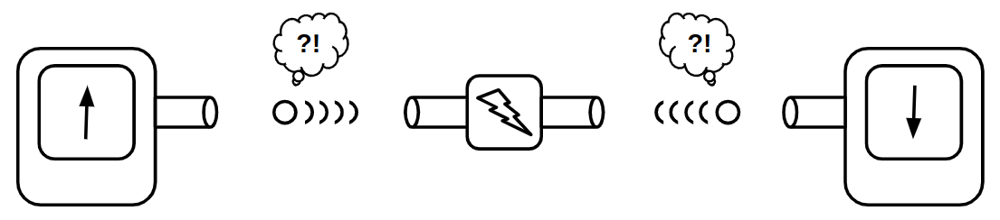
When you actually do this experiment in a lab, you'll always see that the spin of the right and left particles are opposite of each other. Quantum physicist's theory is that, the particles do not have definite spins when they are generated. They only acquire a definite spin when they reach the detector. If that's the case, and their spin is truly random, then how do these particles get opposite spins? If their spin is truly random, they'll have to to talk with each other, telling their spin so that the other particle can get the other spin. If the particles are far from each other, their data-transmission should happen faster than the speed of light.
Einstein, seeing that particles are not obeying his no-faster-than-light law, claimed that the spin of the entangled particles are not random, but their spins are deterministically chosen upon creation, so they don't have to "communicate" with each other. Nobody could prove that Einstein is wrong. Nobody could prove he is right either. In fact, some scientists claimed that this will always remain a mystery, since there is no way to experiment whether the particles know their spin before the measurement or not, until, an Irish physicist named John Stewart Bell designed an experiment that could show which theorem is true!
Fortunately, one doesn't need to know a lot of math and physics in order to understand his experiment. The experiment is as follows:
Imagine, instead of measuring only a single property, we measure three different properties (E.g spin of the particle around three different axis). The results will be similar to the case where we only measure a single axis: the spins of the right-hand-side will be opposite of the respective spins of the left hand side (E.g If the left-hand-side particle's spins are Up-Up-Down, the right-hand-side spins will be Down-Down-Up). Now, instead of measuring the spins in all three axis at the same time, we'll put three buttons on the detectors, allowing us to choose the axis we want to measure the spin in.
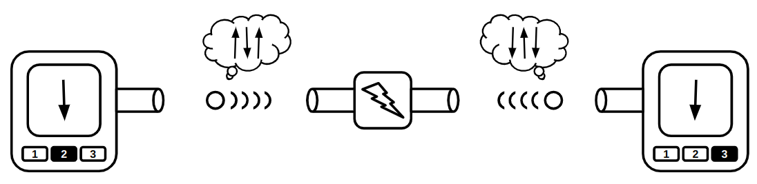
Unlike the previous experiment in which the spin of the left detector and right detector were opposite of each other, now it is possible to observe same spins by the detectors. Now, let's assume that Einstein's statement is true, and the spins of the particles are determined when the particles are generated. Assuming we randomly choose the button on the detectors, what is the probability of observing opposite directions on them? It's simple probability, let's try all different combinations:
[TODO]
It is obvious that in at least \(\frac{5}{9} \approx 55%\) of the experiments, the detectors should show opposite directions. Physicists experimented this and only in 50% of the samples the detectors appeared to show opposite directions. This was a strong proof that we live in The Matrix!
Exploiting the indeterminism
If you are now convinced that we are living in a computer simulation, we can now exploit the fact that some particles in our world do not have definite states, and try to build new types of computers with it, computers than can compute stuff that a simple classical computer just can't, welcome to the world of quantum computers!
Before teleporting to the quantum world, let's first agree on what state means on a classical computer. In a classical computer (E.g the Brainfuck processor we built in the previous sections), a n-bit register may only be in one of the \(2^n\) possible states. In the quantum world however, particles may have indefinite states. A particle may be 50% spin up and 50% spin down. By interpreting those indefinite properties as bits, we may have bits that are both 1 and 0 at the same time! So a n-bit quantum register maybe in all \(2^n\) states as a same time. In other words, an n-bit qunatum register is a probability distribution showing how possible each of the \(2^n\) states are. Let's simulate the a quantum-state as a Python class:
import math
import random


class QuantumState:
    def __init__(self, bits):
        self.bits = bits
        self.values = [0 + 0j] * (2**bits)
        self.values[0] = 1 + 0j

    def is_unitary(self):
        return math.isclose(sum(map(lambda v: abs(v) ** 2, self.values)), 1)

    def apply(self, gate):
        res = []
        for row in gate:
            res.append(sum([row[i] * self.values[i] for i in range(len(self.values))]))
        self.values = res

    def observe(self):
        dice = random.random()
        accum = 0
        for i, p in enumerate(self.values):
            accum += abs(p) ** 2
            if dice < accum:
                s = bin(i)[2:]
                while len(s) < self.bits:
                    s = "0" + s
                return s
        raise Exception()

    def sample(self, times=1000):
        states = {}
        for _ in range(times):
            v = self.observe()
            if v not in states:
                states[v] = 0
            states[v] += 1
        return states
As you can see in the code, a n-bit Quantum register is a list of \(2^n\) complex numbers. We can also assume that quantum-state is a unitary vector (A vector that its length is 1). In order to check if a qunatum-state is valid or not, we have implemented a is_unitary method which calculates the length of the vector, and checks if it is equal to 1.
Quantum-gates are transformations that can convert a unitary vector to another unitary vector. Such transformations can be represented with square matrices! The apply method applies a quantum-gate \(T\) (Which is basically a \(2^n \times 2^n\) matrix) on the gate, resulting to a new state: \(S_{next}=S \times T\)
Lastly, in order to simulate a quantum-state's non-deterministic behavior, we have added a observe which throws a dice (Using Python's random.random() function) and decides what the observed state of the quantum-state is, given the probability distribution.
We can sample the results of the observe function for many times, in order to get more sense of what is happening. We have defined a method sample for this purpose.
Initially, we set the probability of the n-bit quantum-state to be \(000 \dots 000\) for 100% of the time. Thus, if we start sampling a state with no transformations, we will always be in the first state:
s = QuantumState(3)
print(s.sample(1000))  # {'000': 1000}
Here are some gates that can be applied on single qubits:
def not_gate():
    return [[0, 1], [1, 0]]
And there are some
def cnot_gate():
    return [[1, 0, 0, 0], [0, 1, 0, 0], [0, 0, 0, 1], [0, 0, 1, 0]]


def swap_gate():
    return [[1, 0, 0, 0], [0, 0, 1, 0], [0, 1, 0, 0], [0, 0, 0, 1]]
Kronecker is simple: you'll just have to
For example:
\[\begin{bmatrix} 1 && 0 \\ 0 && 2 \end{bmatrix} \times \begin{bmatrix} 1 && 2 \\ 3 && 4 \end{bmatrix} = \begin{bmatrix} 1 \times \begin{bmatrix} 1 && 2 \\ 3 && 4 \end{bmatrix} && 0 \times \begin{bmatrix} 1 && 2 \\ 3 && 4 \end{bmatrix} \\ 0 \times \begin{bmatrix} 1 && 2 \\ 3 && 4 \end{bmatrix} && 2 \times \begin{bmatrix} 1 && 2 \\ 3 && 4 \end{bmatrix} \end{bmatrix} = \begin{bmatrix} 1 && 2 && 0 && 0 \\ 3 && 4 && 0 && 0 \\ 0 && 0 && 2 && 4 \\ 0 && 0 && 6 && 8 \end{bmatrix}\]
def kronecker(a, b):
    return [[val_a * val_b for val_a in row_a for val_b in row_b]
            for row_a in a
            for row_b in b]
If you want to apply a single-bit gate on \(i\)th gate of a multi-bit state, you'll have to manipulate the gate matrix using the following formula:
\(I \times I \times \dots \times G \dots \times I \times I\)
Here is a Python implementation which consecutively calculates Kronecker product of res with 2x2 identity matrix I for n time except when we are in the ith position, which in that case we calculate the product by a 2x2 gate (Resulting in a 2^n by 2^n matrix).
def apply_single_bit_gate_at(gate, i, n):
    assert i < n
    res = [[1]]
    for j in range(n):
        if j == i:
            res = kron(res, gate)
        else:
            res = kron(res, I)
    return res
Now, some of our quantum gates (E.g CNOT and HADAMARD gates) accept two qubits. So we'll also need a function to extend those 4x4 matrices to 2^n by 2^n ones using another function apply_two_adjacent_bit_gate_at. This one accepts a 4x4 matrix as the gate and assumes you want to apply it on two adjacent qubits i and i+1 suitable for a n qubit quantum state.
def apply_two_adjacent_bit_gate_at(gate, i, n):
    mats = []
    skip = False
    for k in range(n):
        if skip:
            skip = False
            continue
        if k == i:
            mats.append(gate)
            skip = True
        else:
            mats.append(I)
    return kron_all(mats)
What if we want to apply a 2-qubit gate on qubits of the state that are not necessarily adjacent? There is a quantum gate named SWAP which allows you to swap the qubits of a 2-qubit state. You can somehow move the qubit to the correct location by periodically swaping it with its neighbor, slowly shifting it to left/right until the two desired qubits get adjacent, and then apply your gate using the apply_two_adjacent_bit_gate_at function, and then again putting back the moved qubit to its original location by swapping in reverse. This is how the implementation will look like:
def zeros(n, m):
    return [[0 for _ in range(m)] for _ in range(n)]

def identity(n):
    res = zeros(n, n)
    for i in range(n):
        res[i][i] = 1
    return res

def matmul(a, b):
    n, m, p = len(a), len(b), len(b[0])
    c = zeros(n, p)
    for i in range(n):
        for k in range(m):
            if a[i][k] != 0:
                for j in range(p):
                    c[i][j] += a[i][k] * b[k][j]
    return c

def apply_two_bit_gate_at(gate, i, j, n):
    if i > j:
        i, j = j, i

    dim = 2**n

    # Step 1: swap j down to i+1
    U_swap = identity(dim)
    for k in range(j-1, i, -1):
        S = apply_two_adjacent_bit_gate_at(SWAP, k,  n)
        U_swap = matmul(S, U_swap)

    # Step 2: apply gate
    U_gate = apply_two_adjacent_bit_gate_at(gate, i, n)

    # Step 3: swap back
    U_unswap = identity(dim)
    for k in range(i+1, j):
        S = apply_two_adjacent_bit_gate_at(SWAP, k, n)
        U_unswap = matmul(S, U_unswap)

    return matmul(U_unswap, matmul(U_gate, U_swap))
Also, notice I introduced some matrix helper functions which can be used for generation, zero and identity matrices. Also, since we want a single gate matrix returned by the apply_two_bit_gate_at function, we are combining all of the needed matrix operations together using a matrix-multiplication function matmul.
In order to test our quantum circuits, we will add two helper functions. The first, basis_state, creates basis states from their numerical representation (e.g., index = 6 corresponds to |110⟩). The second function converts a basis state into a bit string (e.g., given the column vector [[0],[0],[1],[0],[0],[0],[0],[0]], it returns "010" for a 3-qubit system).
We will then create basis states, pass them through our quantum circuit, and convert the resulting state back into a bit string. This will allow us to examine the circuit outputs in a human-readable way.
# Create basis state |index>
def basis_state(index, num_qubits):
    state = [[0] for _ in range(2 ** num_qubits)]
    state[index][0] = 1
    return state

# Bit representation of a basis state
def basis_state_to_bitstring(state, num_qubits):
    active_index = None

    for i, amplitude in enumerate(state):
        if amplitude[0] == 1:
            if active_index is not None:
                raise Exception()
            active_index = i

    if active_index is None:
        raise Exception()

    return format(active_index, f'0{num_qubits}b')
Here we will assume all eight basis-states of a 3-bit quantum state are fed into a circuit that applies CNOT on qubit 0 and 2 of the state. We will then print the binary representations of the before/after states to see if a CNOT is indeed being applied.
NUM_QUBITS = 3

for i in range(8):
    before = basis_state(i, 3)
    print(basis_state_to_bitstring(before, NUM_QUBITS), '=>', end=" ")
    after = matmul(apply_two_bit_gate_at(CNOT, 0, 2, NUM_QUBITS), before)
    print(basis_state_to_bitstring(after, 3))
Here is the output of the code:
000 => 000
001 => 001
010 => 010
011 => 011
100 => 101
101 => 100
110 => 111
111 => 110
As you can see, the first 4 states are intact, because the MSB qubit (Which is the control qubit) is zero, which means a NOT operation should not be applied on the LSB qubit. The last 4 states are clearly showing a qubit-flip in their LSB qubit since the control qubit is 1. This shows our primitive functions are working correctly.
Grover's algorithm
Is a cool quantum computer algorithm that let's you find an input to a function that gives out a specific output using only \(O(\sqrt{n})\) searches. In normal case, when you find to brute-force a function to find for a certain input, you'll have to go through all possible inputs. If there are N inputs, on average, you'll probably need to run the function N/2 times. Something like this:
N = 10000

for x in 0..N:
    if f(x) == desired_y:
        return x
Now what if I tell you, you can find that x by only doing around ~100 searches? That's what Grover's algorithm is all about: brute-forcing a function with significantly less function runs. I mean how is that possible? Well, it's like allowing other computers in parallel universes to do that search for you. But that's not real scientific explanation! Here is a better analogy:
Imagine you have a set of tuning forks with different frequencies. You want to find the one with frequency \(f\). One way is to find your desired fork is to just take them one by one, strike them, and see if it makes the desired sound. That's a O(n) algorithm. Now a smarter approach would be to stand aside those forks, and generate a sound of frequency \(f\). Now, the fork with same frequency will start resonating. You can see that by eyes and find the fork. You didn't even need to strike any of them, the "answer" just popped up to your face. All you needed was shouting the frequency, and the fork just revealed itself.
Now I would say quantum algorithms are somewhat similar. You propagate the "output" you are looking for as a wave, and the correct input to your function that generates the desired output will reveal itself!
def hadamard_all(n):
    return kron_all([HADAMARD] * n)

def grover_oracle(target_index, n):
    dim = 2 ** n
    O = identity(dim)
    O[target_index][target_index] = -1
    return O

def diffusion(n):
    dim = 2 ** n
    D = [[2 / dim for _ in range(dim)] for _ in range(dim)]
    for i in range(dim):
        D[i][i] -= 1
    return D

def grover_search(target, n):
    qs = QuantumState(n)
    qs.apply(hadamard_all(n))
    qs.apply(grover_oracle(target, n))
    qs.apply(diffusion(n))
    return qs

NUM_QUBITS = 3
TARGET = 5  # |101>

qs = grover_search(TARGET, NUM_QUBITS)

print("Final amplitudes:")
for i, v in enumerate(qs.values):
    print(format(i, f'0{NUM_QUBITS}b'), ":", round(v.real, 3))

print("\nSampling:")
print(qs.sample(10000))
Output:
Final amplitudes:
000 : 0.177
001 : 0.177
010 : 0.177
011 : 0.177
100 : 0.177
101 : 0.884
110 : 0.177
111 : 0.177

Sampling:
{'101': 7815, '000': 324, '110': 310, '011': 289, '111': 285, '010': 322, '001': 329, '100': 326}
Why matrices?
The term quantum computer is a bit misleading. In fact, a quantum-computer is a regular classical-computer equipped with a device that can perform operations on a quantum-state (Maybe someday, you’ll be able to connect a quantum-state to your laptop too). For example, the quantum operation could be radiating the “state” with a electromagnetic wave of some frequency. A real quantum computer doesn’t perform matrix multiplications, like what we did in our simulator! Matrices just happened to be good mathematical structures for modeling different quantum operations!
As previously noted, a quantum-state is somehow a probability distribution over its different possible states.
The state is a vector of length one. It’s length will always be one.
In a quantum operation, the final result of one bit is somehow a linear combination of all other bits. That's why quantum operations are defined by matrices, because matrices are just a group of coefficient-rows that are stacked on top of each other. Matrices are a simplified version of "functions". They are some sort of machines that are able to be combined with each other with some nice mathemtical properties. These little creatures are going to be used in other chapters as well.
Hear!
Music of the chapter: Giorgio by Moroder - By Daft Punk
Human senses
Before starting this chapter, I'm expecting you to understand that human brains are biologically evolved computers. They are massive networks of interconnected cause/effect gates, which can dynamically change their behavior (Unlike a silicon computer gate, which has a fixed behavior over time) to learn stuff. These interconnected gates excite each other through electrical impulses. Electrical impulses are the language with which our neurons talk with each other. So, in order to sense something from the external world, some kind of translation is needed, and that's why we have Senses.
Regular computers have sensors too. For example, we can think of a keyboard as a computer’s way of sensing the world. It allows humans to communicate with it, much like ears and eyes allow a human to receive input from the world around them, including other people. It's interesting to know that there are 6 different kinds of ways a human brain can make sense of the external world. Here is a brief list:
| Name | Organ | Stimulus | Stimulator |
|---|---|---|---|
| Sight | Eyes | Light | Physical self |
| Hearing | Ears | Sound | Larynx |
| Balance | Inner-ears | Acceleration | ?! |
| Smell | Nose | Chemical substances | Sweat |
| Taste | Tongue | Chemical substances | ?! |
| Touch | Skin | Position/Motion/Temperature | Touch/Hit |
We used to refer to the human senses as the five main senses, but there are also less obvious types of sensory inputs. For example, there’s something like a gyroscope in your inner ear that allows you to sense rotation and movement through space. This is what lets you feel the acceleration of a car even when your eyes are closed. Similarly, different kinds of pain or bodily sensations can also be considered sensory inputs. The key point is that your brain’s neurons are not only connected to each other, but also to various peripheral systems. These peripherals enable you to function as a complete, integrated human system.
Human brains need to communicate with each other to maximize their evolutionary goals, but they aren't directly wired together. (Imagine if they were actually connected by wires—an interesting question would be: would they then become a single brain? A single "person"?) So, what's the solution? How can a conscious piece of meat, trapped inside a hard skull, communicate with other brains?
Much like the regular computers in your home, human brains also have external auxiliary hardware connected to them, primarily designed to perceive input from other computers—or, in this case, other humans. The eyes, ears, nose, tongue, and skin are examples of input devices connected to the brain, allowing it to sense the effects of the external world.
In addition, there are organs connected to the brain that enable it to produce various outputs or effects in the world. Some examples include generating sound, giving a smile, or even producing attractive scents for mating!
The brain's internal language is the flow of electricity through dendrites and axons. Different parts of the brain communicate with each other via electrical signals. However, for a brain to connect with the external world and transmit data to another brain, a series of cause-and-effect conversions is required. Messages must be transformed into some other form of signal that can travel through the environment, and then be converted back into electrical signals upon reaching the receiving brain.
Imagine you're designing a communication system for human-like creatures that allows them to exchange information through their environment. How would you do it? That's right—the most obvious method is sound: one creature produces vibrations (speech), and another perceives them (hearing). This process is what we know as speaking and listening.
This chapter explores one of the most effective mediums of human communication: sound. Voices, music, and auditory signals have not only shaped human interaction, but also inspired the foundations of modern communication systems.
Today, humans are no longer the only entities that can produce and perceive sound—computers can do it too! You hear digital sounds and voices every day, whether it's a song playing on your laptop, or the sound your phone makes when you press a key. Computers can generate sounds, and more impressively, they can also "hear" them. These sounds don't even have to be mechanical. Your computer, for instance, communicates with your Wi-Fi router using "electromagnetic sounds."
In fact, programming a computer to generate and interpret sound is one of the most exciting and creative things you can do as an engineer.
We’ll begin by exploring the history of sound, starting with the earliest inventions that enabled us to record audio. The good news is that sound waves—the basic building blocks of any sound—can be generated quite easily by a computer. That’s because sound is, at its core, a mechanical disturbance that propagates through the air. There are many ways to convert alternating electrical signals in a wire into mechanical vibrations. And guess what kind of output computers are great at producing? Electrical signals! (Not all human senses are this easy to simulate—smell and taste, for example, are still challenging to reproduce with current technology.)
Along the way, we’ll also take a brief detour into music theory. In fact, understanding music is a fun and intuitive way to start learning about sound. As you progress through this chapter, you’ll discover how you can compose a Beethoven symphony by writing a program that outputs nothing but numbers. Musical notes are like the LEGO pieces of our minds. Putting the right ones in the right order can influence human emotion—evoking sadness, joy, excitement, fear, wonder, and more. Learning how to create music will not only deepen your appreciation for sound, but also make you a better programmer. After all, programming is also about assembling the right pieces in the right sequence to create something meaningful.
Once you’re comfortable generating sound, we’ll shift our focus to how a computer can "hear." You’ll learn that a single sound can actually be a combination of many simpler, "primitive" sounds—and that we can break down complex audio into these basic components. Just like humans, computers can be trained to detect specific primitive sounds within a more complicated mix. We use this principle to build systems that allow computers to communicate with each other through sound.
History of vibration
Thomas Alva Edison—some people think of him as a villain who stole Tesla’s ideas. We're not here to judge. Regardless of the controversy, he was an inventor whose creations had a significant impact on history and inspired many. In this piece, I want to talk about one of his inventions that I personally find both primitive and impressive: the Phonograph (nowadays often referred to as the Gramophone), the first human invention capable of recording and replaying sound.
Sound itself is the result of mechanical waves traveling through the air. In a vacuum, where air (the medium) is absent, sound cannot travel. Humans can produce sound because they have an organ—the larynx—that vibrates the air. These vibrations eventually reach the eardrums of another person, causing them to move in a specific pattern. To record and replay sound, we must capture these air movements and then recreate them in the same way. Phonographs offer a mechanical approach to this problem.
Phonographs, as defined by Wikipedia, are devices that can record and reproduce sound. The idea behind them is both clever and elegant. Imagine a needle on a rotating disk. The needle is connected to something similar to a loudspeaker, which vibrates when someone speaks nearby. As the needle vibrates, it engraves grooves or varying depths into the disk. Over time, as the disk rotates, these grooves represent the air's movement—the sound—captured over that period.
Here’s what makes the phonograph fascinating: after recording, you can place the needle back at the starting position and play it again. This time, instead of engraving, the needle follows the previously cut grooves, causing it to vibrate. This vibration transfers to the loudspeaker, which in turn vibrates the surrounding air. The air vibrations reach our eardrums, which convert the movement into electrical signals understood by our brain—and voilà, we hear the sound again. This reveals something profound: any arbitrary sound can be encoded as a stream of numbers. In the case of the phonograph, the "numbers" are the depths of the grooves engraved into the disk during the original recording.
Phonographs were an early mechanical solution to the challenge of recording and replaying audio. Eventually, people learned to encode sound as electrical signals and invented electrical speakers, which could convert those signals back into air movement. The way an electric speaker works is surprisingly straightforward. It’s essentially an electromagnet—a magnet whose field is generated by electrical current flowing through a coil—placed near a permanent magnet attached to a flexible diaphragm. When electric current flows through the coil, the resulting magnetic field either attracts or repels the nearby magnet (depending on the voltage’s polarity), causing the diaphragm to move. When the current stops, the magnetic field disappears, and the diaphragm returns to its resting position. This is a direct conversion of electrical signals into mechanical vibrations—in other words, sound.
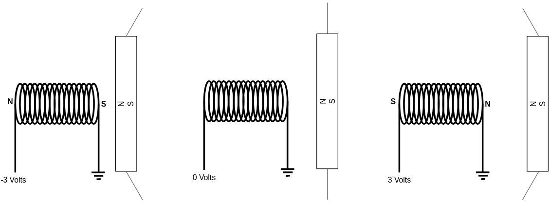
The system surprisingly works in reverse too! (Remember how a phonograph could both record and play music?) Vibrations in the air can cause the magnet—connected to the diaphragm—to move, which in turn induces an electrical current in the coil. Eureka! You can convert sound into a stream of voltages on one side, transmit it through a wire, and play it back on the other side. This is a very basic explanation of how a simple telephone works.
One important detail is that the electrical current generated during recording is very weak and not strong enough to move the magnet and diaphragm on the receiving end. The solution is to amplify the signal along the way.
A similar principle applies to phonographs. The vibration applied to the phonograph needle alone isn't strong enough to vibrate the surrounding air and produce audible sound. Instead, the vibration is routed to a mechanical loudspeaker, where it is somehow intensified before reaching our ears.
(If you're curious about how the amplification process works, stay tuned for Chapter 6!)
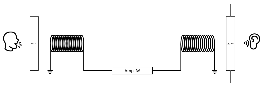
When people speak, a neural process triggers a mechanical response—specifically, the vibration of the larynx. This vibration causes the surrounding air to vibrate as well, creating a wave that travels through the air and reaches the ears of others. In this way, neural activity in one brain leads to neural activity in another, effectively linking minds.
This process forms the basis of a meta-computer we call "society." Human communication acts like neural transistors, enabling the construction of complex systems—essentially large-scale cognitive networks—that are capable of doing remarkably sophisticated and sometimes unexpected things.
Selective hearing
We are now convinced that what we perceive as audio is nothing but a stream of intensities. This intensity can take different forms: mechanical (like the depth of the groove in a gramophone disk), electrical (alternating voltage in a wire), electromagnetic (a disturbance that can travel even through the vacuum of space), or simply a number in a computer. From now on, let's refer to these streams of intensities as signals.
The main question is: why is something as simple as a signal—a single stream of alternating air pressure—such a perfect medium for humans (or even computers) to communicate with each other? The answer lies in our incredible ability to selectively focus on what’s important to us.
Imagine you're at a party, and everyone is dancing to loud music. There's a lot of noise, yet you can still hear what your friend is saying. That’s remarkable because sound is a single signal—a single stream of intensities. The loud music and your friend's voice are combined into that same signal.
The reason you can still make sense of your friend’s voice in a noisy environment is similar to how you can recognize the taste of an energy drink inside a cocktail—even when it contains many ingredients and is “loud” in flavor. This is because we have specialized receptors that detect different primitive elements of a sensory experience, whether it's hearing or tasting. In the case of taste, the primitive elements might be sweetness, sourness, bitterness, etc. Each specific taste is a unique combination of these basic flavors. But what are the primitive elements of an audio signal?
The answer to this is one of the most incredible and important discoveries in engineering. In 1822, French mathematician Joseph Fourier, in his work on the flow of heat, claimed that any function or signal can be expressed as the sum of a series of sine and cosine terms. This means we can treat pure sine waves as the primitive elements of signals. Fourier also introduced a method to decompose any signal into its sine components—what we now call the Fourier Transform.
If you record someone speaking and decompose the recording into its sine components, you'll find that most of the energy lies within a specific frequency range. Different people speak in different frequency ranges. So, theoretically, if one person speaks in one range and someone else in another, our brain can distinguish between them—even if they speak at the same time!
However, if their frequency ranges are too similar, it becomes difficult for the brain to separate the voices. This is why the human larynx has evolved in such a way that most people have distinct vocal frequency ranges.
Let your computer speak!
Enough talking. As I always say, the best way to understand something is to explain it to a computer. In this section, we will learn how you can shake the magnetic plate of the speaker on your computer and use that to create different sounds. As we mentioned earlier, sound can be represented as a stream of intensities. This stream can be stored or generated by a computer as well. Computers generally come with hardware that can take a stream of data as input and smoothly apply it to the magnetic coil of a speaker, causing it to move back and forth. This movement vibrates the nearby air, allowing the computer to produce sound on its own. So, our first step is to find a way to send this data stream to your hardware.
If you have a Linux machine, your life will be easier! There is a program called pacat (PulseAudio Cat) that allows you to directly send sound samples to your computer’s audio device. It operates at a default rate of 44,100 samples per second (which means if you provide 44,100 samples, it applies all of them to the magnetic coil in exactly one second). By default, it reads signed 16-bit integers from its standard input and plays them through your speaker by varying the voltage applied to the speaker’s magnetic plate. When the sample has the lowest possible value (-32,768), the maximum negative voltage is applied and the plate is pulled inward; when the sample has the highest possible value (32,767), the plate is pushed outward. A sample value of 0 means zero voltage, which results in zero magnetic field and the plate remains in its original position.
The obvious implication is: if you give a constant voltage to the speaker, you won’t hear anything. You’ll only start to hear sound when the input stream of numbers fluctuates rapidly, causing the magnetic plate to move back and forth quickly. The faster the changes, the higher the frequency (pitch) of the sound you’ll hear!
Since pacat can accept any data as input, we can try passing non-audio data to it too, just to see what happens! For example, try giving the random data generated by /dev/urandom to pacat:
cat /dev/urandom | pacat
You'll hear random noise! It might be fun to hear the voice of the Linux kernel:
sudo cat /boot/vmlinuz | pacat
Random noise is boring. Now it's the time to generate sounds that actually make sense to our brain. For the beginning, we are going to write a program that can generate sounds of different frequencies. This will become a playground for our experiments and will help us to understand the concepts much better. Throughout this chapter, we'll be generating waves of different frequencies, combining them, manipulating them in weird waves and then hear how it sounds! Let out journey begin!
The formal definition of a wave with frequency \(f\), is something like this:
\(sin(2\pi ft)\)
\(t\) is the variable of time in seconds, and \(f\) is the frequency. Plot this function and you'll see that the function oscillates between -1 and 1, for exactly \(f\) times during 1 second.
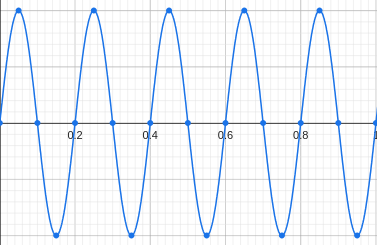 { width=250px }
Since \(t\) is a real number, there are infinite possible values for it (Even in a limited range like \([0,1]\)). We can't apply infinite different voltages to our magnetic plate in a finite time. A solution is to increase \(t\) with an fixed number, and take a sample out of the function. How fast we take samples from our function determines our sampling rate. A sampling rate of 100 means that we are taking 100 samples per second. In order to reach sampling rate of 100, we have to increase \(t\) by 0.001 everytime we take a new sample. The sampling rate should be high enough so that we are able to generate a wide range of frequencies, otherwise it'll become useless. A sampling-rate of around ~40000 is enough to be able to generate sounds that are hearable by a human.
A very standard sampling-rate for sounds is 44100. pacat uses it by default too. The next step is to substitute the \(t\) variable with \(\frac{n}{44100}\) where \(n\) is the sample number: \(sin(2\pi f\frac{n}{44100})\), then we should just create a loop in which the value of \(n\) by 1 (Effectively causing the value of \(t\) increases by \(\frac{1}{44100}\))
import sys
import struct
import math


# Send sound sample to stdout as a 16-bit signed integer
def put(x):
    sys.stdout.buffer.write(struct.pack("h", int(x * 32767)))


sample_rate = 44100  # Rate per second
step = 1 / sample_rate
length = 5  # Seconds
freq = 440


def f(t):
    return math.sin(t * 2 * math.pi * freq)


t = 0
for _ in range(sample_rate * length):
    put(f(t))
    t += step
put(x) function is getting a floating point value \(-1 \leq x \leq 1\) as its input and putting a signed short integer between \(-32768 \leq s \leq 32767\) into the stdout. It is the main gate which allows us to convert an electrical cause to a mechanical effect, by vibrating a magnetic plate in your computer!
Redirect your script's output to the pacat program and hear the voice of your program:
pacat <(python3 music.py)
Frequency combos!
Remember that each arbitrary signal can be assumed as nothing but composition of sine waves? A fascinating fact is, our ears are actually able to recognize the existence of two different frequencies in a single signal, and we can actually experiment that! Instead of defining our f(t) function as a single sine, we can embed two sine components in a single signal by adding them together:
def f(t):
    a = math.sin(t * 2 * math.pi * 440) * 0.5
    b = math.sin(t * 2 * math.pi * 660) * 0.5
    return a + b
We are multiplying a and b by 0.5 so that the output value remains between -1 and 1, otherwise the value of a + b may go below -1 or above 1, which doesn't make sense to our audio device. When you apply a coefficient to a signal, the sound will remain the same, only the energy/intensity of it (Its volume), will decrease/increase! Here we are halving the volume of our original sine function so that some space remains for the other sine component.
If you hear this function, you will actually notice that it consists of two sounds. Your brain can successfully decompose the output wave into two sounds, and this is amazing! The reason that you can recognize the 440Hz and 660Hz sound in the output of this script is the same reason you can hear your friend in a loud room full of noise, your brain is able to decouple sounds with different frequencies.
Invent your sound pallete!
Now that we are able to generate sounds of different frequencies, I want you to do an experiment. Try generating frequencies that are of the form \(2^nf\). E.g. try hearing these frequencies: \(440, 880, 1760, 3520, \dots\)
def f(t):
    if t < 1:
        return math.sin(t * 2 * math.pi * 440)
    elif t < 2:
        return math.sin(t * 2 * math.pi * 440 * 2) # 880Hz
    elif t < 3:
        return math.sin(t * 2 * math.pi * 440 * 2 * 2) # 1760Hz
    elif t < 4:
        return math.sin(t * 2 * math.pi * 440 * 2 * 2 * 2) # 3520Hz
In the code above, we are generating different frequencies through time. We start with 440Hz, and we double the frequency every 1 second.
Hear them carefully, and then compare how they sound when their frequency is doubled. Try a different coefficient. Generate sounds that are of the form: \(1.5^nf\): \(440, 660, 990, 1485, \dots\)
We can discover something very strange and important here. Sounds that are generated when the frequency is doubled each time, are very similar to each other (At least, to our brain). While in the second experiment, sounds seem to be different with each other. If the sounds that are generated in the first experiment are similar, then what makes them different?
Let's try another experiment (This time without coding!). Play one of your favorite musics and try to sing on it. Try to sing on it with lower and higher pitches. Even though you have changed your voice, your singing still "fits" the song. By singing on a song with higher pitch, you are not actually shifting your frequency by some number, but you will actually multiplying it by a power of two. A man and woman with totally different frequency ranges can both sing on the same song, but both of the singings will "fit" on the song, as long as the frequencies are multiplies of powers of 2. I think it's now safe two say, frequencies that are doubled (Or halved) every time, have same feelings.
Let's start with 300Hz. We calculate powers of two multiplied by the base frequency. Here is what we get:
..., 37.5Hz, 75Hz, 150Hz, 300Hz, 600Hz, 1200Hz, 2400Hz, ...
Although there areLet's agree that they are all basically the same "sound", and let's put a name on them. Let's call them sound number 1 or S1.
Whatever frequency we take from the range 300Hz-600Hz, there will also exist the corresponding "same-feeling" sound in ranges 75-150, 150-300, 600-1200, 1200-2400 and etc.
Conversely, we can also conclude that any random frequncy have an corresponding "same-feeling" frequency in 300Hz-600Hz range. In order to find its same-feeling frequency, we just need to halve/double it, until it gets between 300Hz-600Hz. (E.g. let's start with 1500Hz, we halve it 2 times and we get 375Hz which exists in the range, so 375Hz is the equivalent same-feeling sound of 1500Hz). We know there are infinite number of frequencies between 300Hz-600Hz. A single S1 is not enough for creating beautiful pieces of music. We could only build Morse codes out of the single sounds! So let's discover and define other sounds in the same range.
Imagine we define S2 as a sound that is in the middle of two S1s. Given that the self-feeling sounds are repeated in a loop, here is what we should expect:
S1 - 75Hz
S2 - ?Hz
S1 - 150Hz
S2 - ?Hz
S1 - 300Hz
S2 - ?Hz
S1 - 600Hz
S2 - ?Hz
S1 - 1200Hz
What is the definition of middle? Let's say, \(C\) is in the middle of \(A\) and \(B\), when the distance between \(C\) and \(A\) is equal with the distance between \(C\) and \(B\). How is distance defined in case of frequencies? As a first guess, we can take the average of two S1 frequencies in order to find the S2 frequency.
S1 - 75Hz
S2 - (75 + 150)/2 = 112.5Hz
S1 - 150Hz
S2 - (150 + 300)/2 = 225Hz
S1 - 300Hz
S2 - (300 + 600)/2 = 450Hz
S1 - 600Hz
S2 - (600 + 1200)/2 = 900Hz
S1 - 1200Hz
As you can see in the calculations, you can get other S2 sounds by multiplying/dividing any S2 sound by powers of 2, just like what happened with S1. So the derived S2 frequencies are all valid and all same in terms of their feelings.
This is not the only way one can define the "middle" frequency here. Imagine instead of taking the average, we multiply the numbers, and take their square-root instead. This is called an "multiplicative" average, or a geometric mean (As opposed to an arithmetic-mean that we used in the first example):
\(m=\sqrt{ab}\)
We know that the frequencies are doubled in each iteration, so \(b=2a\). Substituting this in the equation we get: \(m=\sqrt{2a^2}=a\sqrt{2}\)
S1 - 75Hz
S2 - 75 x sqrt(2) = 106.06Hz
S1 - 150Hz
S2 - 150 x sqrt(2) = 212.13Hz
S1 - 300Hz
S2 - 300 x sqrt(2) = 424.26Hz
S1 - 600Hz
S2 - 600 x sqrt(2) = 848.52Hz
S1 - 1200Hz
As you can see, both of these definitions of "middle" give us valid sounds (By valid, I mean they are frequencies that are same-feeling), that indeed are in the middle of the S1 frequncies. The first definition of "middle" gives us numbers that have same arithmetic distance with the S1 frequencies (\(m-a=b-m\)), while in the second definition, the results are numbers that have same multiplicative distance with the S1 frequencies (\(\frac{m}{a}=\frac{b}{m}\)). Unfortunately, each of these defintions of middle is giving us different middle frequencies.
So, the million dollar question is, which one is the more appropriate defintion of "middle" here?
Let's look to those numbers again, this time without considering the middle frequencies. Take 3 consecutive S1s in a row. (E.g 300Hz 600Hz 1200Hz). By definition, if we take 3 consecutive sounds, the second one is in the middle of the first and third sound. If we forget about our artificial middle frequencies and take a stream of S1s as our reference sounds, are the middle frequencies the artithmetic or the geometric mean of the other frequencies?
Let's say our 3 consecutive sounds are \(2^ka\), \(2^{k+1}a\) and \(2^{k+2}a\). How can we calculate the middle frequency if we only had the values for the first and the third frequency? Let's try both artithmetic and geometric means.
\(m_a=\frac{2^ka+2^{k+2}a}{2}=\frac{2^k(a+4a)}{2}=5\times 2^{k-1}a\)
\(m_g=\sqrt{2^ka \times 2^{k+2}a}=2^{k+1}a\)
Obviously, geometric mean is the natural definition of "middle" in a raw stream of S1 frequencies, so it makes a lot of sense to define middle as the geometric mean.
Good to mention that another bug also happens when we try to define middle frequencies with arithmetic means. Although S2 resides in the middle of two S1s, S1s do not reside in the middle of S2s! \(\frac{112.5 + 225}{2} \neq 150\). This does not happen when we use geometric means: \(\sqrt{106.06 \times 212.13}=150\).
Fortunately, we have been able to find a way to halve frequency ranges and create new same-feeling sounds out of them! But are 2 sounds enough for making a song? Well, we don't have to stop here. We can still find the middle of a S1 and a S2 and define a new S3 sound. The middle of the gap between an S2 and the next S1 can also define a new S4 sound. We can build infinitely many sounds just by halving the frequency gaps!
 {width=250px}
Enough explanation. Given that you now know how same-feeling sounds are derived, let's talk about the standard frequencies that are used in the music we hear everyday. Just like how we defined a base frequency S1 for deriving new sounds, music composers also defined a base frequency (That is 440Hz) and derived the other sounds out of it. They called their base frequency A, splitted the gap between two consecutive As into 12 different sounds (Probably because 12 was big enough to make big variations of music and small enough so that the sounds remain distinguishable for human ears) and named the 11 other derived sounds as A# B C C# D D# E F F# G G#. How can you take 12 sounds out of a base frequency? New sounds can be derived by multiplying the previous sound by \(\sqrt[12]2 \simeq 1.05946\). Starting from \(A\) sound, if you do this 12 times, you get back to the next same-feeling A sound again, because \(\sqrt[12]2^{12}=2\).
A = 440Hz
A# = 440 * 1.05946 = 466.16
B = 440 * 1.05946^2 = 493.88
C = 440 * 1.05946^3 = 523.25
C# = 440 * 1.05946^4 = 554.37
D = 440 * 1.05946^5 = 587.33
D# = 440 * 1.05946^6 = 622.25
E = 440 * 1.05946^7 = 659.25
F = 440 * 1.05946^8 = 698.46
F# = 440 * 1.05946^9 = 739.99
G = 440 * 1.05946^10 = 783.99
G# = 440 * 1.05946^11 = 830.61
A = 440 * 1.05946^12 = 440 * 2 = 880
Just like painters, we now have a sound pallete!
Let your computer sing!
Now that we have our pallete of sounds ready, we may start playing simple pieces of melodies! A simple melody consists of musical notes that come, stay for some time and then fade away. There can also be times when no musical not is being played, silence itself is an ingredient of music.
Defining the frequencies of musical notes as a list of constants may come handy in the next sections:
SILENCE = 0
A = 440           # La
A_SHARP = 466.16
B = 493.88        # Si
C = 523.25        # Do
C_SHARP = 554.37
D = 587.33        # Re
D_SHARP = 622.25
E = 659.25        # Mi
F = 698.46        # Fa
F_SHARP = 739.99
G = 783.99        # Sol
G_SHARP = 830.61
We can have a chain of ifs in order to play different notes at different times. Here is an example that goes through the musical notes in a C major scale (We'll have a quick look into the theory of music and scales soon):
# Play Do, Re, Mi, Fa, Sol, La, Si!
def f(t):
    if t < 0.2:
        f = C
    elif t < 0.4:
        f = D
    elif t < 0.6:
        f = E
    elif t < 0.8:
        f = F
    elif t < 1.:
        f = G
    elif t < 1.2:
        f = A
    elif t < 1.4:
        f = B
    else:
        f = SILENCE
    return math.sin(t * 2 * math.pi * f)
Notice that we define SILENCE as a wave with frequency 0.
Instead of defining a melody as a long list of ifs, we may have a list of notes and calculate the index of the note that should be played in any given time by doing a division:
SONG = [C, D, E, F, G, A, B]

def f(t):
    note_index = int(t / 0.5) % len(SONG)
    f = SONG[note_index]
    return math.sin(t * 2 * math.pi * f) if f else 0
We are now ready to synthesize our first melody: let's go ahead and play Twinkle Twinkle Little Star:
SONG = [C, C, G, G, A * 2, A * 2, G, SILENCE, F, F, E, E, D, D, C]
(Note: the reason we are multiplying A by two is that we want the version of A with higher pitch (Or the A note on the next octave), remember the same feeling sounds? We discussed that if you multiply a note by a power of two, you will get the same sound, but in a higher pitch, so effectively, A * 2 is still A!)
Ok, there is a small problem here, the subsequent notes which have same frequency are connecting together. [C, C] doesn't sound like two independent Cs, but it sounds like a long-lasting C. Here is a quick solution:
DURATION = 0.5  # Seconds
WIDTH = 0.8  # 80% of the note is filled with sound, the rest is silence

def f(t):
    note_index = int(t / DURATION) % len(SONG)

    if t - note_index * DURATION > DURATION * WIDTH:
        return SILENCE

    f = SONG[note_index]
    return math.sin(t * 2 * math.pi * f)
Here we are silencing the last 20% of the note duration with silence. This makes it possible for us to distinguish between the notes! Try different WIDTHs to see the difference.
Yins and Yangs
Years ago when I was a high-school student, once our Chemistry teacher wanted take an oral quiz from us. He randomly chose a student, brought him to the blackboard and asked him an unusual question. Why does a proton has positive electrical charge, while an electron has negative electrical charge? Why isn't it the other way round?
The question has a fairly simple answer, negativity and positivity are merely names assigned to these primitive particles, so that we can analyze their behaviors. The question is like asking why humans with male reproductive systems are called men, while humans with female reproductive systems are called women?
Genders and electrical charges are not the only dualities in our universe. In fact, we have infinite concepts in our unverse that has duals. Good and bad, happiness and sadness, light and dark, love and hate, forward and backward, angel and devil, heaven and hell, or even zeros and ones in our computers, they are all examples of dualities.
In many of these duals, one thing refers to the presence of something while the other things refers to the absence of that thing. In context of zeros and ones, we can say one refers to existence of some quantity while zero defines absence of it.
Duals are interestingly two sides of a single coin. A single side cannot exist alone: it can only have a meaning when the other side also exists. That holds true for all other duals. Happiness wouldn't exist if there wasn't any sadness. Positive numbers wouldn't exist if there weren't any negative numbers (If we didn't have negative numbers, our algebra would become bugos).
You can see that many of these interesting phenomena emerge when we try to pull "numbness" from two sides and break it into into two meaninful pieces.
Some of these halvenings are conceptual, meaning that they are not something emerged in our universe like protons and electrons, or women and men. And example is negative and positive numbers, or real and imaginary numbers. We can somehow argue that negative and positive numbers are things that exist even if our universe does not exist.
And some of them are reflections of these conceptual Yin and Yangs. The fact that some living creatures have genders only emerged after millions of years of evolution. In fact many living creatures did not have genders and they split into two only after evolution decided to mimick duality, maybe because duality is good.
You might wonder why I'm saying all this. Well, I thought thinking about duals could be a good starting point for understanding why melodies have feelings in themselves. Why do some of them bring joy, while the other bring sadness?
Recipes of feelings!
Play these two frequency combos with your synthesizer, and think about how you feel about them. If you were supposed two attribute the happy/sad feelings to these sounds, how would you do it?
The first one is a sound composed of three frequencies A, C_SHARP, and E, known as a A-major triad:
def f(t):
    a = math.sin(t * 2 * math.pi * A) * 0.33
    c_sharp = math.sin(t * 2 * math.pi * C_SHARP) * 0.33
    e = math.sin(t * 2 * math.pi * E) * 0.33
    return a + c_sharp + e
The second one is a sound composed of three frequencies A, C, and E, known as a A-minor triad:
def f(t):
    a = math.sin(t * 2 * math.pi * A) * 0.33
    c = math.sin(t * 2 * math.pi * C) * 0.33
    e = math.sin(t * 2 * math.pi * E) * 0.33
    return (a + c + e) * 0.33
Most probably, you will percieve joy when listening to the A-major sound, while feeling confusion and sadness when listening to the A-minor sound. The reason we attribute feelings to musical patterns like these are merely cultural! Music has somehow become an international language among humans, since there are very few nations/tribes in the world who will percieve minor patterns as happy and major patterns as sad. This simple duality (That is somehow made-up by humans!) is one of the most important foundations of what we today know as music!
Sequences may have minor/major feelings too. Play these two sequences of notes and think about how you feel about them:
A_MAJOR = [A, B, C_SHARP, D, E, F_SHARP, G_SHARP]
A_MINOR = [A, B, C, D, E, F, G]
Just like the frequency combos, it's very probable that you'll find the A_MAJOR sequence happy and confident, while the A_MINOR one has a bit of confusion and probably sadness.
If you are already excited about the way a simple note sequence might feel, you might want to try these two:
A_MINOR_HARMONIC = [A, B, C, D, E, F, G_SHARP]
A_MINOR_MELODIC = [A, B, C, D, E, F_SHARP, G_SHARP]
The feelings of both of them are very similar to the A_MINOR sequence, but they have even more confusion, one might even say that these sequences have some kind of "magical" feelings.
You can keep going and expanding the sequences by appending the same notes that are in the next octaves. It's easier to catch the feelings of the sequences this way:
def next_octave(m):
    return [n * 2 for n in m]


SONG = A_MINOR_MELODIC
SONG += next_octave(A_MINOR_MELODIC)
SONG += next_octave(next_octave(A_MINOR_MELODIC))
Now, think of these note not as sequences, but as ingredients which you can use for making melodies. Choose a sequence and cook a melody by picking notes only from that sequence. You will have a melody which can have a happy, sad, confusing or even a more complicated feeling! These sequences, or note-ingredients are what is called by musicians as musical scales. We just explored A-major and A-minor scales.
Now tell me, what is the musical scale of the Twinkle Twinkle Little Star melody we synthesized earlier? Wrong! Although the musical notes that are used in this song are the notes of the A-minor scale, it has a happy feeling, it has a "major" feeling! So what has happened?
To understand what is happening, let's first play the expanded version of A-minor scale again, but this time, we'll cut the first two notes in the resulting sequence:
A_MINOR = [A, B, C, D, E, F, G]
SONG = A_MINOR
SONG += next_octave(A_MINOR)
SONG += next_octave(next_octave(A_MINOR))
SONG = SONG[2:]
Weird, it seems like that the location of the sequence from which we start our sequence has strong effects in the way the melody feels!
The truth is, the resulting sound is not in the A-minor scale anymore. Although it has a major feeling, it's not an A-major (You can compare them). It is a C-major!
C_MAJOR = [C, D, E, F, G, A * 2, B * 2]
What is pattern that makes A_MAJOR and C_MAJOR have same feelings, although using different notes? The truth lies in that ratio the frequecy is increasing!
def ratios(song):
    res = []
    curr = song[0]
    for i in range(1, len(song)):
        res.append(song[i] / curr)
        curr = song[i]
    return res

A_MAJOR = [A, B, C_SHARP, D, E, F_SHARP, G_SHARP]
C_MAJOR = [C, D, E, F, G, A * 2, B * 2]

print(ratios(A_MAJOR))
print(ratios(C_MAJOR))
The resulting lists are both equal, this means that the notes themselves are not important, but the way the frequencies are increasing is what makes these sequences to have special feelings.
We can have functions that can make minor/major scales for us:
HALF_STEP = math.pow(2, 1 / 12)
WHOLE_STEP = HALF_STEP * HALF_STEP

def apply_scale(starting_note, scale):
    result = [starting_note]
    for step in scale:
        result.append(result[-1] * step)
    return result


def minor(starting_note):
    return apply_scale(
        starting_note,
        [WHOLE_STEP, HALF_STEP, WHOLE_STEP, WHOLE_STEP, HALF_STEP, WHOLE_STEP]
    )


def major(starting_note):
    return apply_scale(
        starting_note,
        [WHOLE_STEP, WHOLE_STEP, HALF_STEP, WHOLE_STEP, WHOLE_STEP, WHOLE_STEP]
    )
Now you can make musical scales on the fly!
Chords
Our ears are wonderful. They can distinguish between different frequencies and notes, even when they are mixed up with each other. It might be worth noting that this isn't true for our eyes. Our eyes can't distinguish between the yellow color, and the mixture of red and green colors! (Yes, they are different, and this unfortunate fact isn't that bad: it has made it much easier for us to build color display! More on this in the next chapter)
So if the ears are able to make sense of "frequency mixtures", why not trying to bake new sounds by mixing different frequencies with each other? It'll be like mixing different colors with each other and making new colors!
In the world of music, these mixtures are often referred as "chords". Chords are simply just mixtures of different notes that exist in a certain musical scale. Musicians have found ways to make up chords that feel nice and good. Let's explore a few of them. I would like to start with triads (We already explored the A-major and A-minor triads if you remember): these are chords that are made of 3 different notes. Just like how we categorize musical scales as majors and minors, some triad chords are also categorized in this way too.
Given a starting note, here are some of the triads you can make:
def major_triad(root):
    return [root, root * (HALF_STEP ** 4), root * (HALF_STEP ** 7)]

def minor_triad(root):
    return [root, root * (HALF_STEP ** 3), root * (HALF_STEP ** 7)]

def diminished_triad(root):
    return [root, root * (HALF_STEP ** 3), root * (HALF_STEP ** 6)]

def augmented_triad(root):
    return [root, root * (HALF_STEP ** 4), root * (HALF_STEP ** 8)]
As you expect, minor and major triads have sad and happy feelings, but we have two new patterns here too: diminished and augmented triads somehow sound mysterious, disturbing and some people say melancholic!
Now, you may want to use chords in your music to go above building pure melodies. Not all chords are going to "fit" to the musical-scale your are using in your music! Here is how you can make triads that will sound nice and fit your music: start with a root note in the scale, and also pick the third and fifth notes. E.g in scale of A-major, here are the triads you can use:
- A B C# D E F# G#
- A B C# D E F# G#
- A B C# D E F# G#
- A B C# D E F# G# A
- A B C# D E F# G# A B
- A B C# D E F# G# A B C#
- A B C# D E F# G# A B C# D
Let's automate this and write a function that can generate the triad chords of a given scale for us on the fly:
def triads(scale):
    # The scale is repeated twice to avoid overflows!
    notes = scale + next_octave(scale)
    res = []
    for i in range(7):
        res.append([notes[i], notes[i+2], notes[i+4]])
    return res
[POINTER]
Sometimes we already have a note in a given scale, and we just want to extract the corresponding triad of it:
def triad_of(note, scale):
    scale = scale + next_octave(scale)
    i = scale.index(note)
    return [scale[i], scale[i+2], scale[i+4]]
Now let's substitute the notes in the Twinkle Twinkle Little Star with their corresponding triads, and play the triad notes simultanously on every note. We'll define a new function combo to make it easier for us to play a note-combination given a list of frequencies:
def combo(t, freqs):
    return sum([
        math.sin(t * 2 * math.pi * f) for f in freqs
    ]) / len(freqs)

def f(t):
    note_index = int(t / DURATION) % len(SONG)
    triad = triad_of(SONG[note_index], C_MAJOR)
    return combo(t, triad)
See how richer our output has got!
Our toolset is almost enough for generating random pieces that feel somewhat good to our ears. Given we now have some knowledge on musical scales and feelings, we may even inject our desired feelings to these pieces.
Our brief journey in theory of music has now ended. In the next sections, we are mostly going to study more on the waves themselves.
Storing melodies
It's a shame to limit your synthesizer to the Twinkle Twinkle Little Star melody. You perhaps are more interesed in synthesizing the sound of your favorite music, so perhaps you want your synth to be able to play and synthesize some sort of a standardized format for storing melodies. This way, you'll be able to compose a lot of other melodies which people have made and published over the internet for you! There actually is a very commonly used format for exactly that purpose named MIDI. MIDI (Or Musical Instrument Digital Interface), as defined in Wikipedia: is a file format that provides a standardized way for music sequences to be saved, transported, and opened in other systems. You might challenge yourself to write a MIDI parser and interpreter for your synth, but MIDI is a pretty complicated format, and one might need to read a enormous document before he can implemenet it, so I decided to start with something simpler:
There is a simple file format developed by mobile phone manufacturer Nokie for storing ringtones, named RTTTL. We are going to implement a RTTTL parser since it's a relatively simple format. The RTTTL version of the StarWars theme is something like this:
StarWars:d=4,o=5,b=45:32p,32f#,32f#,32f#,8b.,8f#.6,32e6,32d#6,32c#6,8b.6,16f#.6,32e6,32d#6,32c#6,8b.6,16f#.6,32e6,32d#6,32e6,8c#.6,32f#,32f#,32f#,8b.,8f#.6,32e6,32d#6,32c#6,8b.6,16f#.6,32e6,32d#6,32c#6,8b.6,16f#.6,32e6,32d#6,32e6,8c#6
A RTTTL file is composed of 3 sections, separated by :. Here is the description of each section:
- First comes the name of the song, e.g:
StarWars - Then comes a comma (
,) separated list of parameters:d=4,o=5,b=45dis the default duration of each note (As number of beats)ois the octave which we are inbis the beats per minute.
- And at last we have another comma separated list of notes: e.g:
32p,32f#,32f#,32f#,8b.,8f#.6,32e6,32d#6,32c#6,8b.6,16f#.6,32e6,32d#6,32c#6,8b.6,16f#.6,32e6,32d#6,32e6,8c#.6,32f#,32f#,32f#,8b.,8f#.6,32e6,32d#6,32c#6,8b.6,16f#.6,32e6,32d#6,32c#6,8b.6,16f#.6,32e6,32d#6,32e6,8c#6- For each note, we first have its duration (As number of beats). If there isn't any, then the default one is used.
- Then comes the note
- If there is a
.after the note, it means you should multiply the duration with1.5 - And then comes the octave (Otherwide, the default octave is used)
Here is a function that accepts a RTTTL script and returns a list of notes:
def parse_rtttl(rtttl: str):
    NOTES = {
        "p": 0,
        "a": A,
        "a#": A_SHARP,
        "b": B,
        "c": C,
        "c#": C_SHARP,
        "d": D,
        "d#": D_SHARP,
        "e": E,
        "f": F,
        "f#": F_SHARP,
        "g": G,
        "g#": G_SHARP,
    }
    name, params, body = tuple(rtttl.split(":"))
    params = {p.split("=")[0]: int(p.split("=")[1]) for p in params.split(",")}
    notes = body.split(",")
    res = []
    for note in notes:
        dur, name, dotted, oct = re.match(
            r"(\d*)([a-gA-GpP#]{1,2})(\.?)(\d*)", note
        ).groups()
        freq = NOTES[name]
        dur = int(dur) if dur else params["d"]
        oct = int(oct) if oct else params["o"]
        if dotted:
            dur += dur // 2
        res.append((freq, dur))
    return res
Here are some other RTTTL melodies you might want to try!
GoodBad:d=4,o=5,b=56:32p,32a#,32d#6,32a#,32d#6,8a#.,16f#.,16g#.,d#,32a#,32d#6,32a#,32d#6,8a#.,16f#.,16g#.,c#6,32a#,32d#6,32a#,32d#6,8a#.,16f#.,32f.,32d#.,c#,32a#,32d#6,32a#,32d#6,8a#.,16g#.,d#
Gadget:d=16,o=5,b=50:32d#,32f,32f#,32g#,a#,f#,a,f,g#,f#,32d#,32f,32f#,32g#,a#,d#6,4d6,32d#,32f,32f#,32g#,a#,f#,a,f,g#,f#,8d#
More than Sines!
After playing some melodies by generating different frequencies in a sequence, you might nag that the notes are very pure, emotionless, and not at all close to what we hear when we press a key on a piano, and you are right. We are generating pure sine-waves, meaning that what we hear contains only a single frequency. If you analyze the sound coming out of a musical instrument, you will notice that not only it contains frequencies other than the main frequency, but also the strength of those frequencies change over time.
It's not easy to generate a piano sound using pure sine frequencies, but there are other ways we can oscillate a loud-speaker, letting us to get more creative and generate sounds that are more interesting and weird.
As an example, imagine sharp jumpings to -1 and +1 instead of smoothly going up and down like a sine wave. This will make a square wave that feels very differently. Square-waves have vintage feeling, since the game consoles back then didn't have speakers with enough precision for generating sound with needing smoother movement of the speaker's magnetic plate. All they could do was to sharply pull and push the magnetic plate!
Sounds as gates
Engineering is all about making new things, by gluing already existing things together. When synthesizing a sound, the "things" that are being glued together are math functions that produce intensity samples given time. Let's call these functions samplers.
So far, we have been putting all of the sound sampling logic inside a single f function. In case f was simply generating a sine wave, any change on the frequency of the wave would need direct changes in the definition of the f function. A nicer, more engineer-friendly (!) approach would be to define some primitive samplers and provide toolings for combining them together and making new samplers (Like chapter 1, where we defined transistors as primitive elements and started building logic gates and more complex circuits on top of them). In case of producing sound samples, periodic functions like sine-wave generators are basic enough to be considered primitive. Since these functions are kind of oscillating your speaker, we call them oscillators!
Unfortunately there isn't a single sine-wave oscillator since sine-wave oscillators with different frequencies are different and thus sound different. Creating a new function for each of the frequencies is neither practical nor smart, so, thanks to Python we are able to define a function that is able to get a frequency as an input and return a sampler function as its output!
As an example, here is a sampler-creator function that accepts a frequency as its input and returns a sine-wave sampler as its output:
import math

def Sine(freq):
    def out(t):
        return math.sin(2 * math.pi * freq * t)
    return out
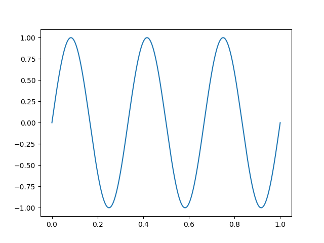 { width=250px }
Now, f can be defined by the output of an oscillator like Sine:
f = Sine(440.0)
See how better it looks? Here are some other forms you can oscillate a speaker. Try hearing them all!
Square
import math

def Square(freq):
    def out(t):
        if math.floor(2 * freq * t) % 2 == 0:
            return 1
        else:
            return -1
    return out
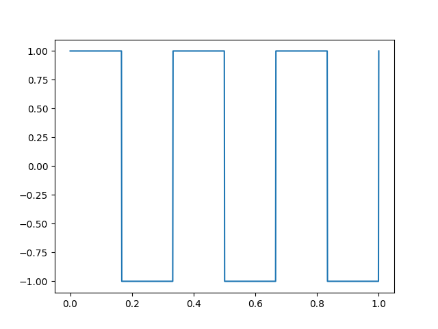 { width=250px }
Sawtooth
def Sawtooth(freq):
    def out(t):
        return 2*(t*freq - math.floor(1/2 + t*freq))
    return out
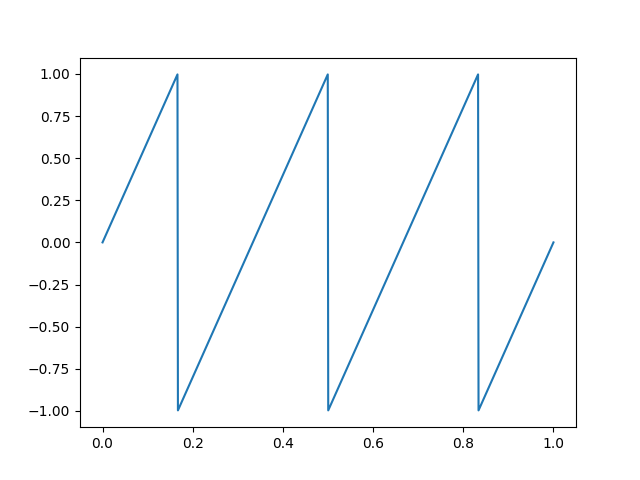 { width=250px }
Triangle
def Triangle(freq):
    def out(t):
        return 2*abs(t*freq - math.floor(1/2 + t*freq))
    return out
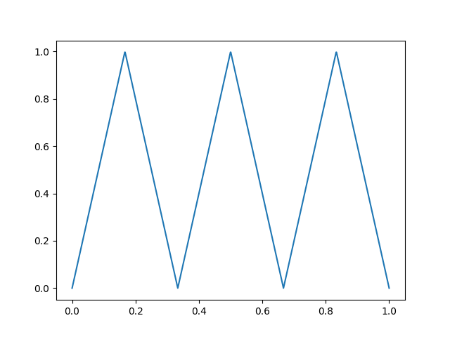 { width=250px }
The gates
In our model of a synthesizer, we assumed that there are some set of primitive samplers, which we can pick as a starting point for building more complicated samplers, thus now we kind of need sampler generators which will accept other samplers as their input. Let's start with a simple example: imagine we want to synthesize a sine wave which has a lower volume compared to the original Sine sampler. We can either create a completely new sampler like LowVolumeSine, or create a general-purpose volume-decaying sampler named Gain, which will accept a sampler as input and returns a new one in which the samples are scaled by some constant:
def Gain(inp, s):
    def out(t):
        return inp(t) * s
    return out
Now, if we want to hear Sine(440.0) with 50% of volume, we would only need to pass it to the Gain sampler like this:
f = Gain(Sine(440.0), 0.5)
Another interesting example would be to get a sampler and apply a coefficient to its input:
def Speed(inp, s):
    def out(t):
        return inp(t * s)
    return out
The following sampler will sound like a 880Hz sound wave, becase we are sampling x2 faster!
f = Speed(Sine(440.0), 2)
When composing a melody, we had to make the notes to stay only for a limited time. Such behavior can be described with a sampler! The mask sampler will get a input sampler, and only allows the first dur seconds to pass!
def Mask(inp, dur):
    def out(t):
        if t >= 0 and t <= dur:
            return inp(t)
        else:
            return 0
    return out
You can also shift a sampler in time:
def Delay(inp, delay):
    def out(t):
        return inp(t - delay)
    return out
The Delay and Mask samplers together can allow you to play a specific sampler, for a limited time, starting at a specific time. The given sampler will start playing a 440Hz sine wave at 5.0s and end in 6.0s.
f = Delay(Mask(Sine(440.0), 1), 5)
Just like the multi-input logical gates we explored in the first chapter, you may also compose a new sampler by combining more than a single sampler. This is where the magic slowly starts to show itself!
def Compose(samplers):
    def f(t):
        v = sum([sampler(t) for sampler in samplers])
        return v
    return f
These three alone are enough for composing melodies:
f = Compose([
    Delay(Mask(Sine(440), 1), 0),
    Delay(Mask(Sine(440), 1), 1.5),
    Delay(Mask(Sine(440), 1), 3),
    Delay(Mask(Sine(440), 1), 4.5),
])
This way of describing a sound is definitely less-efficient (Performance wise) than directly implementing the wave-generator as a plain Python function, but look how manageable and beautiful the code has got. (Perhaps we can achieve the same speed if we write some kind of compiler that is able to translate the modular definition into plain code).
ADSR
Hearing all these compositions of different oscillators, you may still notice that the sounds are far from being pleasant to your ears, and one of the main reasons is that the intensity of those sounds is constant in time, while in real-world, a note gets loud with a delay, and will smoothly lose its intensity as time passes. One way we can bring such effect in our simulation is to actually manipulate the volume of our oscillator through time.
One of those methods, known as ADSR (Attack, Delay, Sustain, Release), assumes that a musical note starts with a volume of 0, quickly reaches its peak volume and then quickly gets down to relatively quieter volume, stays there for a longer time and then starts decreasing its intensity until it reaches zero.
These timings might be different for different instruments, and they do not neccessarrily change linearly. For the sake of simplicity, we will assume the changes all happen in a linear fashion. Here is a graph:
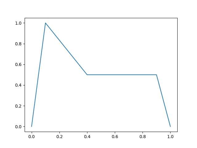 { width=250px }
Fortunately, applying an ADSR effect is as simple as multiplying the ADSR function with the oscillator function!
def Adsr(sampler, a_dur, d_dur, s_dur, r_dur, a_level, s_level):
    def f(t):
        if t < 0:
            coeff = 0
        elif t < a_dur:
            coeff = (t / a_dur) * a_level
        elif t < a_dur + d_dur:
            coeff = a_level - ((t - a_dur) / d_dur) * (a_level - s_level)
        elif t < a_dur + d_dur + s_dur:
            coeff = s_level
        elif t < a_dur + d_dur + s_dur + r_dur:
            coeff = s_level - ((t - a_dur - d_dur - s_dur) / r_dur) * s_level
        else:
            coeff = 0
        return sampler(t) * coeff
    return f
Macro Music Language
Macro Music Language (MML) is a very old and deprecated music description language for storing melodies on computers. MML was originally designed to be used in video games back in 70s, so you probably can't find a lot of software that can play MML files, though I chose to introduce and implement this format since it's fairly simple to implement and there are plenty of music available in this format which you can test your synthesizer with, and unlike RTTTL, it may contain multiple lines of melodies which are played in parallel. Here is a brief spec of this language:
A MML music consists of commands.
cdefgabthe notes. You may get the sharp/flat versions of them by appending#/-respectively. You may also specify the duration as a fraction of the whole note. E.ga2is a half-note andb#8is an eighth note. If a duration is not specified, a default duration is used. If a.appears after the note duration, the duration should be multiplied by 1.5.r/prest/pause! Just like the regular notes it may have a duration as a fraction. E.gp4pauses as long as a quarter note.ofollowed by a number, selects the octave.>,<used for going to the next/previous octave.lsets the default duration for note, as a fraction of the whole note. E.gl8sets the default duration to 1/8 of a whole note.vfollewed by a number, sets the volume of the instrument.tfollowed by a number, sets the tempo in beats per minute.
A MML music may be composed of several lines of melodies which should be played all at the same time. These lines of melodies are separated using &.
Now we would like to write our MML synthesizer as a sampler, just like all samplers we defined in the previous sections. The ComposeMML sampler accepts a MML text, and a instrument as its input, and produces a sampler as its output. The instrument is simply a function that returns a sampler given a pitch.
def simple_instrument(pitch):
    return ADSR(Sine(pitch), 0.1, 0.3, 0.5, 0.1, 1.0, 0.5)

def ComposeMML(mml, instrument):
    return Compose([
        # ...
    ])
Frequency Modulation
One of the interesting sounds you can try to generate is the sound of a siren. A siren is a device that can generate a loud sound, with alternating frequency. The frequency is alternated itself in a sine pattern. Assuming the sound's frequency alternates between \(f_1\) and \(f_2\), we can calculate frequency, by time, as follows:
\(f=f_1 + (f_2-f_1)\frac{sin(t) + 1}{2}\)
We already know altering the intensity of a sound is as simple as applying a coefficient to its sampler function. If you multiply the above function with an oscillator, its volume will alternate. Knowing that we can generate sine wave with frequency \(f\) with \(sin(2.\pi.f)\), you may conclude that the sound of a siren can be modeled by substituting \(f\) with the alternating \(f\) formula:
\(sin(2.\pi.(f_1 + (f_2-f_1)\frac{sin(t) + 1}{2}))\)
Try to generate and play this sound. It will sound weird, not at all like a siren. But why?
If you want to understand why this weird sound happens, try plotting the formula we came up with.
[IMG]
It looks strange, right? Just multiplying the frequency function by \(2\pi t\) doesn’t really work—and that actually makes sense. If the frequency (f) is constant, everything is fine. The input to the sine function just keeps increasing, so you get a normal wave.
But if the frequency changes over time, things break. The input to the sine can sometimes go backward instead of always moving forward. That’s a problem, because a sine wave doesn’t make sense if its input decreases—time should always move forward.
So instead of changing the input directly, what we really want to change is how fast time moves forward. That “speed” is the frequency, and it should always stay positive.
What we’re trying to get is just a sine wave that smoothly shifts between high and low pitch—like a siren.
The correct way to do this is: \(\cos\left(2\pi \int f(t),dt\right)\)
For example:
\(f(t) = f\)
\(f(t) = f_{\text{base}} + f_{\text{alt}} \cos(t)\)
The reason we use an integral is simple: we need to keep track of everything the frequency has done up to time (t). So we add up all the past values of (f(t)), and use that as the input to the sine.
If you plot just that inside part (the integral), it becomes much clearer what’s going on.
[TODO: Frequency modulation]
How can we emulate an ear in a computer
\(X_k=\sum\limits_{n=0}^{N-1}{x_n.e^{-i2\pi kn/N}}\)
Reverb, sound tracing and …
Have you ever heard the echo of your sound in a mountain? Or any echo chamber, like a church? Not only can you hear yourself back, but also the reflected sound has a very fuzzy, dreamy, spritual and psychedellic effect, making it a perfect ingredient for musicians to add to their music. The effect is also known as reverbation, and is pretty common in many style of music we hear nowadays. The fact is, the musicians are not recording their music in echo chambers, thanks to the advancements of electronics and signal processing algorithms, the sound does not have to be reflected in a chamber. We can trap the sound inside an electrical wire, or even a computer simulated chamber, and allow it to chaoticly reverb.
Reverbation is perhaps the most complicated and exciting part of building an audio synthesizer, and here we are going to implement a very simple version of it!
Sound is data
Electromagnetism
Sounds are the result of vibrating air propagating through space. Sound is a kind of wave. When you disturb a still water from some point, the disturbance will start propagating from that point. A cause on a point will have effects on points far from the original point. Just like water (Or any other liquid), waves can be propagated through gases too. Waves are a very important mean of communication. Humans mainly use sound waves for communication. They disturb the air by vibrating their larynx, and the diturbance will propagate in air until it reaches the ears of the listener. Computers can communicate through sound too. Using what you have learnt so far, you can write programs that can encode data as sound and send it through the air to another computer.
Since the sounds we make are propagated through air, without air, we won't able to speak with each other. If you put two people in a vacum space, all they'll see is their friend's lips moving without hearing anything! That's why astronomers communicate through walkie-talkies with each other!
World is a strange place, besides particles and materials, there are non-mechanical things too. Even wondered what prevents two magnets with same poles to get close to each other? If you try to get them close, you'll feel there is "something" in between them, but there actually is nothing. It turns out that moving that "thing" (As the result of moving the magnet), can disturb the area around it too, just like when you move inside water.
Here's another way to think about it: Imagine your entire body is floating in the water in a swimming pool. Assume that the water is completely still, and it will remain so as long as you also remain still and don't move any part of your body. A very slight movement of your hand will create a disturbance in the water (in this case, the water represents the context). Your hand's disturbance will start propagating and reach all parts of the pool. The effect is not immediate, and it will take some time for the motion to reach other areas of the pool. If you start vibrating your hand with some frequency, you will soon see that a slighter vibration (with the same frequency) will begin happening in other parts of the water. The farther the destination point, the more time it takes for the motion to reach, and the less powerful the vibration will be. The very same thing happens in the air. We are all floating in a pool of air, and any movement in the air will have effects on the way air moves. That's why we can communicate with each other. In this case, the context is "air."
Now, there exists a more unusual kind of context in which waves can occur. We can assume that space is filled with some kind of unknown matter that gets distorted when magnets/electrons move through it. This is the context where electromagnetic waves can propagate. This is the context which our cell-phones, wireless networks, gps satellites, remote controls communicate through. The disturbances in this medium are propagates with speed of light, and that’s one of the reasons why we building our computers to communicate through sounds ( which propagate through air, with a speed of 300ms, a lot less than the speed of light)
Metals are also isolated environments in which certain kind of waves can propagate. Imagine having two wires, connected to a power source with a voltage of 5V. Assume we slowly decrease the voltage to 0. The fact is, the effect is not immediate, and the decrease in voltage will reach the end of the wire with some delay!
Einstein claimed that there can’t be anything faster than light [TODO]
If you even remove the sun from the solar system, the earth will keep orbiting around the missing sun for about 7 minutes, [TODO]
Heinrich Hertz, the German physicist, was the first to prove the existence of electromagnetic waves (that's why the unit of frequency is Hertz). James Clerk Maxwell (we'll learn more about his work in the next chapters) predicted the existence of such waves even before Hertz. However, Hertz was the first to show that they truly exist. He accomplished this by capturing the transmitted waves through an antenna he built himself. It's amusing to know that Hertz believed his invention was worthless and had no use, as he said:
"It's of no use whatsoever... this is just an experiment that proves Maestro Maxwell was right—we have these mysterious electromagnetic waves that we cannot see with the naked eye. But they are there."
It's challenging to imagine our world nowadays without his invention. Hertz's story is a good example that demonstrates the potential and impact of studying seemingly useless science in our lives.
Hertz's transmitter and antenna were straightforward, and you can build one yourself if you're curious enough.
Although your computer can generate electromagnetic waves in specific frequency ranges (such as WiFi and Bluetooth), unfortunately, it's not possible to generate arbitrary electromagnetic waves. I always wished there was a way to generate electromagnetic waves by putting wave samples on a wave generator hardware (just like what we do with audio). There are good reasons why manufacturers have not included hardware for that in your computer. If you could generate arbitrary waves, you could interfere with many government-controlled facilities, including national television and radio.
Waves are waves, whether mechanical or electromagnetic; they all share very similar traits. The most important and useful feature of a wave is its ability to transfer data.
Studying waves and how you can utilize them to connect people together is a fascinating topic in both computer and electrical engineering. As I always say, experimenting is the best way to learn. So, throughout the next sections, we are going to experiment with waves using an easy-to-generate kind of wave. We know that it's not possible to generate electromagnetic waves with your computer, and we have also seen how easy it is to generate sound waves. Therefore, we will stick to sound waves and try to transfer different kinds of data between computers through sounds!
Distribute sound, radio stations
Sound is the primary medium of communication for humans, but unfortunately, speaking becomes ineffective when your audience is far away, and the reason is that sound waves lose energy as they propagate in the space. The world was a very different place before the invention of telecommunication technologies. The only way you could communicate with your beloved ones (Who were far away), was to send them physical letters. In the best case, your letter could be delivered in the time it took to transfer a physical object from you to your destination (Which was not very fast obviously). There are faster things in universe by which you can transfer messages of course, light is an example. Lights are also waves, just like sounds, but unfortunately we can't "hear" electromagnetic waves, so we can't use them directly, as a medium of "verbal" communication. We can try to design an intermediary language for translating sentences to visual effects and vice versa. The simplest example of such protocol, is some coding technique known as Morse codes.
Invented in the 1830s by an American artist, Samuel Morse (Yes, sometimes artists are pioneers of technology), Morse code is a method for encoding/decoding latin-alphabet letters into a series of signals (Electrical or visual). It is worth noting that Morse-codes are designed in a way such that the most frequent letters in latin-alphabet have shorter signal representations.
 { width=250px }
Hearing with your computer
PulseAudio's pacat program lets you to put raw audio samples on your computer's speakers. On the other hand, there is another program parec which allows you to record audio samples. pacat puts whatever it gets through stdin on your computer's speaker, while parec puts audio samples it gets through your computer's microphone on stdout. Using these commands together you can record and play audio:
parec > record.wav
pacat < record.wav
Another interesting thing to experiment is to pipe the the parec's output into pacat. Spoiler alert! Your voice will be echoed:
parec | pacat
Now let's try to pass the parec's input through a filter that we'll write in Python, and hear its output via pacat:
parec | python3 filter.py | pacat
Here is a simple filter that allows only half of the samples to go through (filter.py):
import sys, struct

def get():
    return struct.unpack('h', sys.stdin.buffer.read(2))[0] / 32767

def put(x):
    sys.stdout.buffer.write(struct.pack("h", int(x * 32767)))

while True:
    get() # Skip one sample
    put(get())
You will hear a high-pitched version of your voice! (Since skipping the waves-samples will make the waves in the input sound to seem like they are alternating two times faster).
By skipping one of the samples per every two sample, we were able to halven the length of the sound, increasing the speed and frequency of the input sound by a factor of two.
Looking carefully, by skipping the samples, what we are actually doing is taking the samples like this:
\(out[i] = in[2i]\)
Changing the coefficient to 3, makes our input sound 3 times faster. but what if we want to make it only x1.5 faster?
\(out[i] = in[1.5i]\)
Unfortunately, all kinds of digital signals which we process in a computer are discrete, meaning that they are sequences of numbers, the result of sampling the signal over a fixed interval, and you don’t directly have the signal in between two intervals. Although we don’t have the signal data between two intervals, we can predict them with a good accuracy! A very simple prediction model assumes that the distance between two consecutive samples goes through a line!
In other words, you can assume that \(inp[5.5] \simeq \frac{inp[5] + inp[6]}{2}\)
So far, we have had done a lot of experiments using the pacat command, and now it's the time to see what can be done if we allow other computers to receive wave-samples. We have learnt to compose sounds, now its time to decompose them! Putting samples on your computer’s speaker allows you to make disturbance in the air around your computer’s speaker. The disturbance, as seen in the previous sections, will propagate in the space finally reach your ears and you will hear it. Computers can hear those disturbances too, through microphones. Using these two devices together you can build protocols with which computers can talk with each othrr, without any wire connection.
The disturbance doesn’t necessarily need to happen in the air, for example you can basically build devices that can disturb the water in a pool in one side and build a device to detect and listen to the disturbances in the other side of the pool. Using these two, two computers may communicate with each other through water waves!
In real world, what your computer is generating is an electrical signal that is given to a speaker. You can connect the exact same wire to other things too. In fact:
- Connect that wire to a speaker, and the data will propagate through air.
- Connect that wire directly to the destination computer, and the data will propagate through the electrons in the wire.
- Connect that wire to an antenna, and the data will propagate through space.
- Connect that wire to a light-emitter within a optical fiber cable, and the data will propagate through visible light.
Fourier Transform
Fourier-Transform is a method/algorithm by which you can extract frequencies within a wave-form. Remember we could generate sounds that were compositions of two sine-waves with different frequencies? When hearing those sounds, your brain is able to successfully recognize the presence of two different frequencies in what it hears, and that is actually why we are able to understand what someone is saying in a crowded environment with a lot of noise. Our brain is able to focus on a certain frequency (Which is the frequency-range of your friend's larynx). If our brains are able to decompose sounds by their frequency, it's reasonable to think that computers can do that too. Fourier-Transform is the answer. Given a list of signal samples, it will tell you what frequencies are present in that signal. Here is an example:
import cmath  # Math for complex numbers
import math
import matplotlib.pyplot as plt


def fft(x):
    N = len(x)
    if N <= 1:
        return x
    even = fft(x[0::2])
    odd = fft(x[1::2])
    T = [cmath.exp(-2j * cmath.pi * k / N) * odd[k] for k in range(N // 2)]
    return [even[k] + T[k] for k in range(N // 2)] + [
        even[k] - T[k] for k in range(N // 2)
    ]


def get_freqs(x):
    result = [abs(v) / (len(x) / 2) for v in fft(x)]
    return result[: len(x) // 2]


def sine(freq, t):
    return math.sin(2 * math.pi * freq * t)


def sampler(t):
    return sum(
        [
            sine(440, t)
            + 5 * sine(1000, t)
            + 2 * sine(2000, t)
            + 0.5 * sine(9000, t)
            + 8 * sine(16000, t)
        ]
    )


samples = [sampler(t / 32768) for t in range(32768)]
freqs = get_freqs(samples)

plt.plot(freqs)
plt.show()
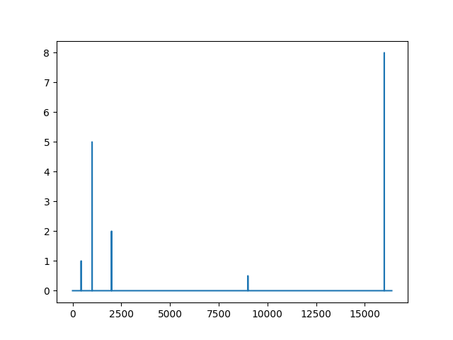
Assuming our sample-rate is \(2^n\), the \(get_freqs\) function will get an array of size \(2^n\) (The signal samples), and will return an array of size \(2^{n-1}\). The \(i\)th element of this array tells your the presence of a sine wave with \(i\)Hz frequency in your input signal. Don't believe it? We can do an experiment, we can actually loop over the frequencies, generate the sinusoids according to their phase and magnitude, and then reconstruct the original frequency:
N = 32768
samples = [sampler(t / N) for t in range(N)]
fft_result = fft(samples)

res = [0 for _ in range(N)]
for freq, val in enumerate(fft_result):
    phase = cmath.phase(val)
    magn = abs(val)
    for i in range(N):
        res[i] += magn * math.cos(2 * math.pi * freq * i / N + phase) / N * 2
Although the code above verifies the fact that the FFT algorithm really works, it's very inefficient (The computation complexity is \(O(n^2)\) because of the nested loops). In fact, you can use the FFT algorithm itself (Which is of order \(O(n.log(n))\)) in order to get back from the frequency-domain into the original signal:
def ifft(x):
    fft_conj = fft([n.conjugate() for n in x])
    return [n.conjugate() / len(x) for n in fft_conj]
The reason that the output array has half of the number of elements in the input array comes back to the fact that, in order to be able to recognize a signal of frequency \(f\), you need to at least have \(2f\) samples of that signal (E.g you can't recognize a 20000Hz frequency in a signal, if your sample-rate is 30000).
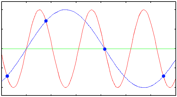
Humans are able to hear sounds with frequencies as high as around 20000Hz, that's why the typical sample-rate for audio files is something around twice of 20000. (A sample-rate of 44100 is pretty popular!).
Dummiest Modulation Algorithm Ever (DMAE)
Assuming that we can generate waves of a single frequency in one machine, and recognize the existence of that exact frequency in another machine, let's try to design an algorithm to transfer data through audio, by encoding the bits into sound waves on one sides, and decoding them, converting back the audio waves into bits on other side (The encoding/decoding parts are usually referred as Modulation and Demodulation).
Let's start by simply generating a sine wave of frequency \(f_d\) (Data frequency) when we want to transmit a 1, and avoid generating it when we want to transmit a 0. On the other computer, we will listen to the sound samples and perform a fourier transform on them. Whenever we recognize a \(f_d\) frequency, we will output a 1, and otherwise a 0. Obviously, we have to agree on a fixed time interval by which bits are sent, otherwise we wont know how many consecutive 0s (Or 1s) are meant to be received in case the receiver is the presence/absence of \(f_d\) is being detected for a long period of time.
As an extra feature, we would like to let the other machine know whenever we have finished sending our data. Right know, we will probably stop generating any sound when there are no more bits to be sent. The receiver machine is not able to know whether we are out of bits, or we are just sending a lot of 0 bits. A simple solution to that problem is to include another frequency \(f_e\) in our generated signal, which is only generated when there are data to be sent.
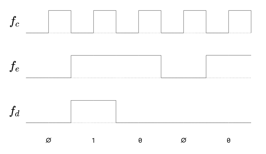
In this case, the receiver will only accept bits when the \(f_e\) frequency is also present in the received signal (Besides presence or absence of data frequency).
Noises, noises everywhere...
Unfortunately, the air is full of noises, if you start speaking while two computers are transmitting data through audio, the disruption may corrupt data, leading unwanted data to be sent on the destination computer. Even the echo/reflections of the sound in the environment may have negative effects (Remember, all waves share similar traits, reflections happen for electromagnetic waves too)
There are methods and algorithms by which you can detect and correct errors in data transfers.
For the sake of simplicity, we won’t discuss error correction. We will try to provide an effective way for error detection, and ask the sender computer to resend the data in case it detects errors.
If you have some knowledge of data-structures, you probably have heard of hash-functions, which are building blocks of hashmaps and hashsets. Hash function are function that get inputs of arbitrary size and give out outputs of fixed size. The special thing about a hash-function is that a slight change in their input has massive effect on their output, and it's hard (And almost impossible, in case we are speaking about crypto-graphically secure hash function, discussed in chapter 5) to find an appropriate input that result in a specific output.
Hash functions (Atleast the idea behind them!) can be useful for detecting errors that happen on data transfers. It's simple, just append the hash of the data to the data you are going to send. The receiver will cut the postfix for you, hash the data and will then check if the hash matches with the postfix. If there is a mismatch, then either the data or the hash itself has got curropted, and the receiver may ask the sender to retransmit the data. (The request to re-send the packet can be carried through the same communication medium we used for sending the data. Packets may also have numerical identifier, so that the receiver can tell the sender exactly which packet got a hash mismatch)
Now, imagine the sender transfers gigabytes of data and the receiver detects an error (It's very very probable when transferring large pieces of data). Isn't it overkill to ask the sender to send the entire data again? Of course not. A better idea is to chunk the data into smaller pieces and detect the errors and ask for retransmission of the smaller parts. In fact, that's the main reason why data in our modern networking infrastructures is sent through packets,
The method described for detecting errors is very inefficient and is not what really happens inside our networks, but the idea is almost the same. After applying the mentioned idea to our sound modulator/demodulator software, we'll have a very error-prone communication medium. Try sending a computer image through sound, it'll probably take hours but it'll work perfectly!
Telephone revolution
When talking about the invention of telephone, many people will give all the credit to the Scottish-born inventor, Alexander Graham-Bell, while just like many other inventions, telephone has a long history too, which includes several names. Graham-Bell was not the first one who had the idea of building a device which could transmit voice through a wire. One of the notable people who worked on a similar idea was a German inventor named Johann Philipp Reis, who invented the Reis telephone, 15 years before Graham-Bell. Unfortunately, Reis died before he could be credited for the invention of telephone.
Reis considered his invention as a device for transmitting music, so he termed his microphone the 'singing station'. Very similar to a phonograph, the Reis telephone was based on a vibrating needle that could increase/decrease electrical resistance between two contacts, which could lead to generation of a electrical disturbance/signal, traveling through a wire. It's very interesting to know that phonographs was invented after telephone (1877)!
In a phonograph, the vibrations made on the needle was causing mechanical effects on a spinning disk. In the Reis'es telephone, those vibrations were causing electrical effects in a wire. Both of these effects could be later/farther be played by a receiver through a speaker. In case of a telephone, the receiver would just amplify those electrical effects, causing vibration in the air, restoring the sound.
Alec Reeves - inventor of pcm 1930s
James Russel - 1978 - store music on optical
Hdd 1956 IBM
Digital data transfer samuel morse early 19th
1950 computers connected dedicated communication lines
Information
Our world is continuos (At least it seems to be) but our computer can only work with discrete data.
- The number of pixels our cameras can capture in a fixed area is limited
- The frames we capture per second in a video-camera is limited
- The audio samples we capture in a microphone is limited
- ...
These limitations cause interesting phenomena: have you ever seen video recording of helicopter rotor blades? Or anything that spins very fast? In some of those recording you may see the blades spinning very slowly, or not spinning at all, or even spinning in reverse! This happens due to the fact that we are limited in the number of frames we're capturing per second. Suppose it takes 10 milliseconds for our camera to take a new frame, and it also takes exactly 10 milliseconds for the spinning object to do a full spin. When the camera takes the new frame, the spinner has already made a full rotation and is back in its original position, so it looks as if it has not spinned at all. Now, slightly increase the rotation speed of the spinner, the spinner will start moving, but very slowly. Decrease the rotation speed and now it looks as if it's spinning in reverse!
It's interesting to know that human eyes do not have "frame-rates". They don't work like video-cameras. Whatever you perceive with your eye stays in your brain for a very short period of time, even if you move your eyes and look at something else, the previous thing you were looking at is still there, but it is just fader. It turns out that pictures take around 1/16 seconds to completely fade away from your eyes, even if you stop looking at them, which somehow means, what you see is the average picture of what you were looking at in the previous 1/16 seconds. Thus if you look at a spinning blade directly through your eyes, you will see something blurry, instead of perceiving it as if it's not rotating, like a video camera.
Another kind of aliasing effect happens when you try to take a picture of something with a lot of alternations, like a net!
If your video-camera is able to capture 60 frames per second, you can't tell if the blade is spinning at:
- 0 RPS, or 60 RPS in reverse
- 10 RPS, or 50 RPS in reverse
- 15 RPS, or 45 RPS in reverse
- 29 RPS, or 31 RPS in reverse
- Generally: \(n\) RPS, or \(60-n\) RPS in reverse
If you don't believe this, here is a proof:
- We know that the camera captures a new frame every \(\frac{1}{60}\) seconds.
- Let's assume the blade spins at speed 15 RPS. Thus the blade does a complete rotation every \(\frac{1}{15}=\frac{4}{60}\) seconds. This means that, when a frame is taken, the blade has gone \(\frac{1}{4}\) rotation.
- Let's assume the blade spins at speed 45 RPS. Thus the blade does a complete rotation every \(\frac{1}{45}=\frac{\frac{4}{3}}{60}\) seconds. This means that, when a frame is taken, the blade has gone \(\frac{3}{4}\) rotation. This also looks like as if the blade has rotated in reverse for \(\frac{1}{4}\) rotation!
This is definitely some kind of data-loss! Unless you are completely sure that the blade does not rotate in reverse, or you are sure that it does not spin faster than 30 RPS. Extracting a general rule out of this: If you are sure that the blade you are capturing a video of spins no faster than \(n\) RPS, then, in order to accurately tell the speed and direction of the spin speed through video, your video camera has to capture at least as fast as \(2n\) frames per second.. Formally speaking, the sampling rate (Here, the samples are frames) should be at least twice of the maximum frequency. This is known as the Nyquist rate and is one of the most fundamental facts of a beautiful category of science known as Information Theory.
Zeno's paradox
Zeno's paradoxes are a series of arguments made by greek philosopher Zeno, which tries to illustrate the problematic concept of Infinite divisibilty in space and time. All of these paradoxes are actually trying to tell us the same thing (If we are not being strict)
Here is one of those paradoxes which you may have heard of before:
Suppose Atalanta wishes to walk a path. Before she can reach to the destination, she must get half-way there, and before reaching to that point she must go \(\frac{1}{4}\) of the way, and before that \(\frac{1}{8}\) of the way, and so on. Seems like, she has to perform an infinite number of tasks in order to move, which Zeno believes is impossible
Humans love to store and copy. If you can copy or store something, you can transfer it. You can write your thoughts on a letter and then give it to your lover to read
Humans dream: being able to share their past experience to the present and future. To the people that are not near them. To people in the future even after they physically die, because life has evolved in a way to keep you alive as long as possible, sometimes the conceptual version of you, and not the physical you. That’s probably why people proudly compromise their lives for something they believe in, because it will make them eternal. Life is strange.
See!
Music of the chapter: Video Killed The Radio Star - By The Buggles
Vision is my (Or probably all people's) favorite way of sensing the world. Imagine out of 6 humans senses, you only could have one of them, which one would you choose?
Vision allows you to find stuff around you, even when they are far enough that you can't access them by your hands. It guides you to things in a physical environment. It shows you the wild animal a coming to you before it's too late.
History of colors
Human eyes are 2d-arrays of electromagnetic receptors that can recognize electromagnetic waves inside the visible spectrum, which are waves with wavelengths of 380-700 nanometers, or in terms of frequency, waves with frequencies of 400-790 terahertz. Theoritically, of you pick a magnet, and and shake it 400,000,000,000,000 times per second, you will see red light coming out of it. Shake it even faster and it will become violet, after that, it will become ultra violet which is not visible by human eyes.
Before studying how an human eye works, let's design one for ourself. As you may already know, electrical flows run a biological neural network. So external inputs need to be translated into electrical signals before they can be understood by your brain. We can use a linear mapping for this conversion. We can map the visible specturm into a voltage between 0.0 and 1.0, where 0.0 is red and 1.0 is violet:
\(e=\frac{f-400tHZ}{390tHZ}\)
Unfortunately, this mapping doesn't explain how black and white colors are represented in a brain. Well I have to tell you something. Black and white colors do not exist. (Or even light-red and dark-blue colors!) They are imaginary colors our brain has invented for itself in order to perceive darkness (Black) and presence of all waves (White). Well I have some bad news. A light beam doesn't necessarily have a single frequency in it. It can be a combination of multiple frequencies, and our mapping can only handle a single frequency. so we need a different represantation for a color of a pixel. A very naive solution is to have a lot of sensors sensing the strength of different frequencies in the visible spectrum for each pixel. I.e. we can have a set of sensors \(e_{400}\), \(e_{401}\), ..., \(e_{790}\), that can measure the presence of different frequencies (And the neighbour frequencies) as a voltage between 0 and 1. In this model, when all frequencies are 0, the brain will perceive it as black. When all frequencies are 1, the brain will perceive it as white. The problem with this model is that it will need a lot of cells for each pixel. If the human eye is a \(n \times n\) array, then we'll need \(n \times n \times 390\) cells in order to perceive an image.
We can get smarter than that. Imagine there are only two sensors per pixel, one will tell you how close the frequency is to \(f_a\) and another will tell you how close you are to \(f_b\) (Imagine \(f_a=500tHZ\) and \(f_b=600tHZ\))
If you are ok in math, you probably know that we can build such behavior using the exponetiation of the absolute difference. (Or squared difference, like a Gaussian distribution equation)
\(e_a = s.e^{-abs(\frac{f - 500}{50})}\) \(e_b = s.e^{-abs(\frac{f - 600}{50})}\)
Now let's try different frequencies in this scheme (Let's assume the strength \(s\) of all frequencies is \(1\)):
\(f=0\) then \(e_a \simeq 0\) and \(e_b \simeq 0\) \(f=500\) then \(e_a = 1\) and \(e_b \simeq 0.13\) \(f=550\) then \(e_a \simeq 0.36\) and \(e_b \simeq 0.36\) \(f=600\) then \(e_a \simeq 0.13\) and \(e_b = 1\) \(f=1000\) then \(e_a \simeq 0\) and \(e_b \simeq 0\)
It's much easier for a brain to analyze differences between outputs, rather than memorizing different values
Now let's take advantage of this design and hack it! Let's say I have two light bulbs, one can emit \(500tHZ\) lights and one can emit \(600tHZ\) lights. Is there a way I can convince the eye that it is seeing a \(550tHZ\) light? Yes! Instead of emitting a \(550tHZ\) light with strength \(1\), I can emit a \(500tHZ\) light of strength \(\simeq 0.32\) and a \(600tHZ\) light of strength \(\simeq 0.32\) at the same time. This will make \(e_a = e_b \simeq 0.36\) which are the same values needed to convince the brain it is seeing a \(550tHZ\) light!
Now the brain's algorithm can be something like this:
- If both \(e_a\) and \(e_b\) are zero, then there is no color (Darkness, infrared or ultraviolet)
- If \(e_a\) is much higher than \(e_b\) then the color is orange.
- If \(e_b\) is much higher than \(e_a\) then the color is green.
- If \(e_a\) and \(e_b\) are relatively equal, then the color is yellow.
Enough imagination! These numbers and formulas are all invented by me to explain the concept. Let's talk about the actual design of human eyes. So the human eyes is designed very much similar to the artifical eye we designed in the previous section. The only difference is that the human eye has receptors for 3 colors instead of 2. I'm sure you can guess what these three colors are! Red, Green and Blue. This fact was discovered in 1802 by Thomas Young (British polymath) and Hermann von Helmholtz (German physicist). They argued that there are 3 kinds of photoreceptors (Now known as cone-cells) in the eye, and they also mentioned that these cells have overlapping response to different wavelengths, allowing our brains to also recognize colors in-between red, green and blue wavelengths. They also mentioned that human eye is not perfect, because it is not able distinguish between yellow, and a mixture of red and blue. If our brains were able to distinguish between those two, it would be much much harder to build computer screens that we have today (Might be even impossible!). That's when God says, this is a feature, not a bug! It's also kind of sad that we are actually blind since our vision (Even in the visible specturm) is very limited and we can only observe very few combinations of light waves.
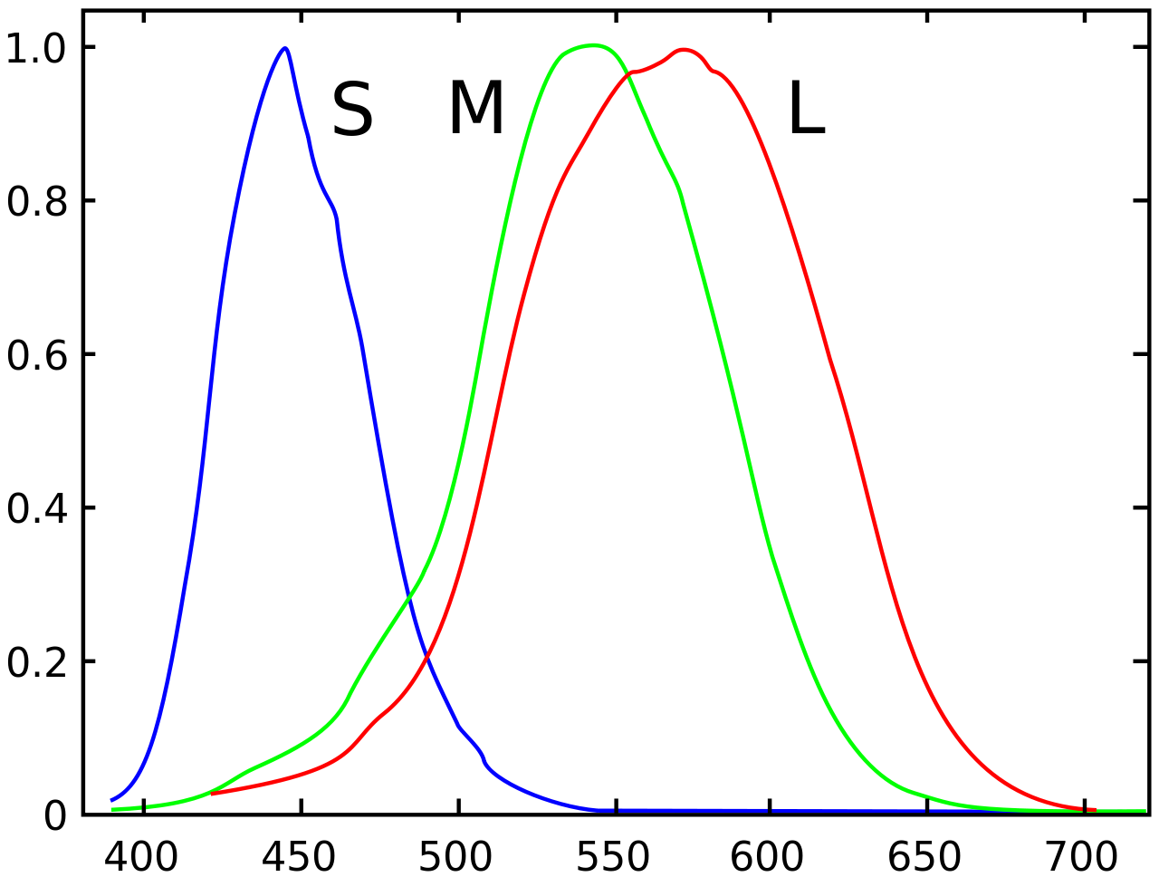
The trade-off
Light and sound, are both results of disturbances that propagate through different contexts. They are both waves, the former is electromagnetic, and the latter is mechanical. So, if they are actually are very similar to each other, why don't we listen through our eyes and see through our ears? Isn't that theoritically possible? Well, not only theoritically, it is even technically possible to see through hearing! You may already know that part of the bats\ navigation strategy depends on producing high-frequency sounds and hearing them back (Notice how similar the generated sound is with a light-source!). Humans have themselves built devices that can see through hearing. The sonography machine, which is used for taking pictures from the inside of your body, is basically a 2D array of ears which can "see" by litting your body with ultrasonic waves and hearing them back.
There are probably reasons the evolution has not decided to make humans hear through electromagnetic waves:
- If that was the case, the sun (Or any other light-source) could disrupt human communications (Imagine hearing the sun!)
- Nature has not been able to find a way to convert neural impulses into electromagnetic waves (I.e it has been very hard for the nature to build a electromagnetic larynx!)
Also, light is much faster than sound, that's why you can see mountains that are hundreds or even thousands of kilometers away from you and be sure that what you see is not something from the past (That's not the case with sound. Even the sound of thunderstorms surprisingly take seconds to reach to our ears). Also, since we need light-sources for seeing stuff, hearing through sound would also need "audio-sources". There isn't a gigantic source of audio on the earth helping us to see through hearing, that's why bats need to produce sounds themselves in order to see their surroundings. Even if humans could produce the audio needed for seeing themselves, it would take enormous amount of energy in order to produce sounds strong enough that could reach places that are thousands of kilometers away. Sun spreads its wave everywhere for free, so why bother seeing through sound? Mechanical waves are just not good candidates for vision.
Besides all these, there is also another big difference between an eye and an ear:
- A human ear is a single wave-receiver that is able to decode a large specturm of frequencies (20Hz-20000Hz)
- A human eye is a 2D array consisting of many wave-receivers that are able to decode very limited number of frequencies (Only three, red, green and blue! But with some tricks, as we discussed in the previous section humans are able to distinguish between electromagnetic frequencies in the range of 400THz-790THz)
A funny analogy: ears are like CPUs, they have a single core (cochlea!) that is able to execute (hear) many kinds of instructions (frequencies) whereas eyes are like GPUs, they consist of many cores (photoreceptors) that are able to execute (see) a limited set of instructions (frequencies). Strangely, GPUs are for calculating pixels that will reach to the corresponding photoreceptor of your eye!
Memento
Years later, in 1826, a french inventor named Nicéphore Niépce had the dream of recording scenes of real life. Back then people knew that there are some chemical compounds that make chemical reactions when they are exposed to light. The chemical reaction would convert the compound to a different compound which fortunately had a different color. The more intense the light is, the stronger the chemical reaction is, applying stronger color changes to the compoound. Nicéphore took advantage of this, he made a plate coated with such a compound and put it inside a camera obscura. A camera obscura was a dark, isolated room with a small hole (Filled with a lense) on one side that projected the image of the outside on the wall. Nicéphore put his coated plate on the wall, and let it be there for a few days. After a few days, the image of the outside started to appear on the plate, which is the very first photography ever done in the world. The resulting picture wasn't perfect (What did you expect?) but the experiment was revolutionary enough to inspire other inventors for building the modern photography.
James Clerk Maxwell, you probably have heard his name before, because of the electromagnetic equations he discovered before, was only 24 years old when he discovered the importance of the trichromatic theory that Young and Helmholz proposed in 1802. The three-colour method, first proposed by Maxwell, was a method for taking colour photographs, given the fact that human eye is only sensetive to 3 ranges of colours. Redness, greenness, and blueness.
He argued that if we take three photographs of the same scene, one with a filter that only passes red light, one that only passes green light and one that only passes blue light, and then somehow combine these three photographs together on a plate, our eyes will be hacked to see a coloured version of that scene. 6 years later, he made the very first colour photography of the history.
You probably already know that when coloured movies came out, old fashioned movie makers were skeptical of them. Good to know that photographers back then also resisted to take coloured photos, but history has shown us that nobody can fight against advancement of technology.
Digital era
Over a century passed before humans invented digital photography, and a lot of inventions and discoveries happened in between (E.g. people started to take pictures in very high speeds and record "movies"), and I would like skip the history and advancements of the analog photography industry in the next 100 years, because there are too many details that are unrelated to the core idea, and start talking about the digital era, the time when people started to store vision on a computer.
It's good to know that digital scanners came before digital cameras. It's also kind of obvious that they have a much simpler structure than digital cameras. The very first digital scanner was invented in 1957 by an american engineer named Russell Kirsch. His scanner could scan photos of size 5cmx5cm in the resoluion of 176x176 pixels (30976 pixels, i.e. ~30 kilopixels!). The bit-depth of his scanner was only 1-bit! The pixels could only be complete black or complete white, so there were no intermediate shades of gray.
In order to deeply understand how digital photography works, you first have to know there exist some materials that their electrical resistance change when they are exposed to light. They are called photoresistors. Their resistance typically decrease when they are exposed to light. So, if you connect a battery to them, when there is no light, no/small current will flow. But when there is light, current will flow. The more intense light is, the more current it will flow. Now how can we use this to measure light intensity of a physical point? Imagine we emit light to a black surface. A black surface will reflect no light, so a photoresistor nearby won't get excited. A white surface will reflect all the light. so the photoresistor will get excited and current will flow. Now imagine we have an electrical circuit that measures the electrical current in a photoresistor. If current is higher than a threshold \(t\), it will output 1, otherwise it will output 0.
What Russell Kirsch did in 1957, was something like this: He made a photoresistor that could move on a 2D grid with electrical motors. It would start on the point \((0,0)\) and scanned a complete row, by moving little by little (In case of a 5cmx5cm area, the distance between pixels is 5cm/176, which is around 0.28mm. Then it would move to the next row and scan another line of pixels. It would output 0 or 1 for each pixel. His scanner was so simple so it couldn't scan grayscale information. But he did a trick. Remember there was a threshold \(t\)? He scanned a point several times with different thresholds, (E.g. \(t=0.1\), \(t=0.2\), \(t=0.3\), ...) then he stored number of times he got the 1 output. This way, he could recognize how white a pixel is and store grayscale information too, without much change in the original design! Kirsch's very first digital scanning is one of the most important pictures taken in the history of photography.
Digital cameras are not scanners. It takes a very long time to takes photos by moving a photoactive subtance and taking samples from it. So what's the solution? Well, naively thinking, instead of a single photon sampler (Photoresistor or ...), we can have and array of a lot of them. In case of Kirsch's design, instead of one moving photoresistor moving on a 2D grid, we can have a plate of 176x176 (30976) photoresistors laying on a 2D grid, which can scan the whole thing in a single step. This design has a very important issue, and the issues is that we might need millions of wires coming out of such a plate, in order to get the outputs of all this resistors (Imagine we want to take a very high resolution image!), which is practically impossible. Engineering is all about giving solutions to challenging problem!
12 years later, in 1969, two Bell Labs physicist named George Smith and Willard Boyle invented the very first Charge-Coupled Device, while working on solutions to improve video-telephone technology. They sketched the first design of a CCD in an hour or so. CCDs are the main elements of modern digital photography. Just like our proposed design, they consist of an 2D array of very small cells that convert light causes to electrical effects. A very common technique is used in order to minimize the number of wires coming out of such an array. Instead of taking a wire out of every cell and reading the content of the cell directly, the cells are interconnected to each other through a single wire that passes through all the cells, and pass their contents to their neighbors in each time step (Shift-registers are used in order to store and pass the data). The CCD will actually output the contents of the image through one line, in a serial fashion.
Applying the trichromatic theory and Maxwell's colour photography idea, we can take colored digital photos too. There exists physical filters that you can put on a CCD array, allowing the neighbouring cells to independently capture the redness, blueness and greenness of a point. They are called Bayer filters. Sometimes, instead of putting a Bayer filter on a CCD array, they natively integrate 3 different CCDs on a CCD array, each of which take the RGB values for each pixel. The method is called, 3-CCD. Obviously using a Bayer filter has a much simpler design.
Anatomy of a computer image
Knowing all this history and human anatomy, we can now tell that a computer image is a 2D array of pixels, where each pixel has 3 properties, red, green and blue. Typically, each color component can have 8-bit value (0 to 255). When the value is 0, that color component is completely off and when the values is 255, it means that color component has highest possible intensity. When all three components are 0, the pixel has complete darkness so we see it as black, and when all of them are 255, we see white (Our brains will be tricked that we are seeing all of the possible waves of the visible spectrum, but we are only seeing three colors!)
It is obvious that a colored computer image can be stored using \(W \times H \times 3\) bytes. (\(W \times H\) pixels, each having three 8-bit components). In order to get comfortable with digital computer images, we are going to manipulate and generate them. Since we don't want to bother ourselves with details of computer image formats (There is so much to learn about how PNG, JPEG and etc works), we are going to use a very simple file format named PPM (Portable PixMap) that emerged in 1980s. PPM stores the image in raw format and doesn't do any compression, that's why it's very simple to generate and manipulate these files. The only metadata that this file format holds is the width and height of the image.
Here is a spec of this file format:
P6 800 600 255
[800x600x3 bytes of data]
A PPM file starts with the magic string P6, then comes a width (As an ASCII string), then the height and then the maximum value of a color component. The metadata values are separated using whitespaces. After the metadata, there comes a whitespace and then we'll have the raw image data. In the example above, we are describing a 800x600 image in which each color component is between 0 to 255. It is worth noting again that the metadata comes as a human readable ASCII string and not bytes. The size of final file is:
P6 (2 bytes) + whitespace (1 byte) + 800 (3 bytes) + whitespace (1 byte) + 255 (3 bytes) + whitespace (1 byte) + raw image data (1440000 bytes).
Before generating the PPM file, let's first create a Python class for storing colors.
class Color:
    def __init__(self, r, g, b):
        self.r = max(min(r, 1), 0)
        self.g = max(min(g, 1), 0)
        self.b = max(min(b, 1), 0)

    def __add__(self, other):
        return Color(self.r + other.r, self.g + other.g, self.b + other.b)

    def __mul__(self, other):
        if type(other) is Color:
            return Color(self.r * other.r, self.g * other.g, self.b * other.b)
        else:
            return Color(self.r * other, self.g * other, self.b * other)
Here colors are represented as tuples made of 3 components, each representing the intensity of the red, green and blue components as a floating point number between 0 and 1. In the constructor, we make sure that the component values will never get above 1 or below 0. We have also implemented the addition and multiplication operators for colors. We'll soon see when colors should be multiplied or added to each other in the next sections.
Assuming our generated image is stored as a 2D array of Colors, let's write a function in Python which is able to save a PPM file given the array:
import io

def save_ppm(rows):
    with io.open("output.ppm", "wb") as f:
        f.write(f"P6 {len(rows[0])} {len(rows)} 255\n".encode("ascii"))
        for row in rows:
            for col in row:
                f.write(bytes([int(col.r * 255), int(col.g * 255), int(col.b * 255)]))
In this function, the rows argument should be a list of height number of rows, in which each row has width number of pixels (tuples) of RGB triads. As an example on how to use this function, let's generate a 800x600 image that all pixels are red:
def color_of(x, y, width, height):
    return (255, 0, 0) # Always return red


WIDTH = 800
HEIGHT = 600
rows = []
for y in range(HEIGHT):
    row = []
    for x in range(WIDTH):
        row.append(color_of(x, y, WIDTH, HEIGHT))
    rows.append(row)

save_ppm(rows)
In order to make our future image generations easier, instead of calculating the color of the pixel directly in the loop, I made a function called color_of which returns the color of the \((x,y)\)th pixel in an image of size \((width, height)\). Currently, this function only returns red, so you may not see anything special in the output, but try this function instead:
import math


def color_of(x, y, width, height):
    xx = x / width
    yy = y / height

    r = (math.sin(x / width * 100) + 1) / 2 * 255
    g = (math.cos(x * y / height / width * 100) + 1) / 2 * 255
    b = (math.sin(y / height * 100) + 1) / 2 * 255
    return (int(r), int(g), int(b))
See what it generates, try different functions and play with it a bit. Guess how shocking it was for computer scientist back then to be able to generate vision using code. That opened doors for insane amount of creativity and the event was big enough to call it a revolution in my opinion!
Control over your screen
What your operating system does to show all of those application windows and user interfaces on your screen is simply repeatedly generating the correct RGB values that represent the current state of your screen and transferring them to your monitor.
On Linux systems, there is a "framebuffer", which is a part of your RAM mapped to your computer screen. Your operating system (or even you!) can manage it directly. Curious how you can manipulate it yourself? Let’s try putting random bytes on your monitor’s pixel buffer and see what happens!
- Press Ctrl + Alt + F1 to switch to a console that is not controlled by a window manager. (A window manager is the software that decides what gets drawn on your screen.)
- Fetch random bytes from
/dev/urandomand write them to your machine’s video buffer:sudo dd if=/dev/urandom of=/dev/fb0
Tada! You should now see random noise on your screen.
It doesn’t have to be random, though!
Emitters vs Absorbers
We are now convinced that the white color does not actually exist, and what we see and define as white is actually a combination of red, green and blue colors. Try litting a surface with red, green and blue light sources, what you will end up is white. But have you ever tried making the white color by combining red, green and blue paint colors? If you have experience in painting, you'll know that the white paint color cannot be made of other colors. In fact, by combining red, green and blue paint colors, you will end up with black! So, what is happening here? What make light sources and colored materials different?
A blue light-source looks blue, because it emits electromagnetic waves in the frequency range of the blue color, whereas a blue object looks blue, because it absorbs all visible electromagnetic waves, but the bluish ones!
By combining red, green and blue light-sources, you will end up with a combination that contains all three frequencies at the same time, so it looks white.
By combining red, green and blue paint colors, you will end up in some color that absorbs all visible electromagnetic waves, thus it looks black.
Drawing a line
Drawing a circle
Why do we use electrical cause effects? Because they are small and fast, and can easily be routed by metal wires Fastest cause effect type is light
Having fun with the pixels
When learning computer graphics, before jumping to complicated algorithms like 3D rendering, there are some other stuff you can do to leverage your power of manipulating pixels.
There are plenty of things you can draw on a 2D surface. Let's start with drawing a simple 2D line. A 2d line may be defined by its slope and offset:
\(y = ax + b\)
Given two points, you can find the corresponding \(a\) and \(b\) that passes through this line too. Assuming the points are: \(P_1 = (x_1, y_1)\) and \(P_2 = (x_2, y_2)\):
\(a = \frac{y_2 - y_1}{x_2 - x_1}\)
\(b = -ax_2 + y_2\)
Let's have a class for working with lines!
class Line:
    def __init__(self, slope: float, offset: float):
        self.slope = slope
        self.offset = offset

    def get_y(self, x: float):
        return self.slope * x + self.offset

    @staticmethod
    def from_points(a: Vec2D, b: Vec2D) -> Line:
        slope = (b.y - a.y) / (b.x - a.x)
        offset = -slope * b.x + a.x
        return Line(slope, offset)
Here is something interesting to draw with simple lines:
[TODO]
Circle
A circle can be defined given its center and radius. Just like the Line class, we may also have a Circle class:
class Circle:
    def __init__(self, center: Vec2D, radius: float):
        self.center = center
        self.radius = radius
Beauty of symmetry
Human beings invented numbers merely to count stuff. They weren't aware that the same numbers could someday help us to explain the universe, and build the foundations of the technology we have today. So it may now make sense why ancient people were mostly performing addition, subtraction and multiplications with numbers and nothing more. A strange fact is that, negative numbers (And even the number zero!) made no sense to ancient people.
So when did people realize there is a need for numbers other than \(1, 2, 3, \dots\)? A potential answer to that question is that human beings love symmetry. Symmetry is an important factor in determining how beautiful something is. The fact that there is an answer for \(5-3\) but \(3-5\) made no sense (To the ancient mathematicians) was kind of annoying. It would make math more solid and beautiful if there was an answer for \(3-5\). It would make the subtraction operator symmetrical. So people said, why not? Let's just assume numbers below zero exist, and call them negative numbers!
Negative numbers are not the only made-up constructions that have made math and its operations more symmetrical. The symmetry we are going to talk about in this section is a new kind of numbers called imaginary or complex numbers. Perhaps the most obvious reason why imaginary numbers had to be invented is the Fundamental Theorem of Algebra. The theorem simple claims that any degree \(n\) equation has exactly \(n\) roots. E.g, for any degree-2 (Quadratic) equation there exactly exists 2 answers/roots.
Take this equation as an example:
\(x^2 + 3x - 10 =0\)
This is a degree-2 equation that obeys our assumption: it has two roots: \(-5\) and \(2\). The polynomial can be decomposed into two degree-1 polynomials: \((x+5)(x-2)\). More generally, it looks like that, any degree degree-n polynomial is in fact the result of multiplying \(n\) degree-1 polynomials like this: \((x-\alpha_1)(x-\alpha_2)(x-\alpha_3)\dots(x-\alpha_n)\). But that's not the case with some polynomials. For example:
\(x^3 + x^2 - 7 x - 15=0\)
A valid answer to this equation is \(3\), but no matter how hard you try, you can never find the second and third root of the equation with the regular numbers we are used to.
\(x^3 + x^2 - 7 x - 15=(x-3)(x-\alpha_2)(x-\alpha_3)\)
Just like how we solved the asymmetry of the subtraction operator by inventing negative numbers, let's make something up to ensure our math remains symmetric! The result is, a new kind of numbers known as complex numbers!
Just imagine
As you know, you can extract the solutions of a quadratic equation using this magical formula: \(\frac{-b \pm \sqrt{b^2-4ac}}{2a}\). A quadratic equation will stop having regular solutions when the term inside \(\sqrt{b^2-4ac}\) becomes negative. That's because the square root of a negative number is meaningless. But just imagine that the square-root of negative numbers do actually exist, but we just don't know them yet (Just like we didn't know the existence of negative numbers). Based on our knowledge of the square-root operator, we know that: \(\sqrt{ab}=\sqrt{a}\times\sqrt{b}\). Based on that, we can say that the square-root of a negative number is in fact the square-root of a positive number, multiplied by square-root of \(-1\):
\(\sqrt{-a}=\sqrt{-1}\times\sqrt{a}\)
That's right, we extracted a primitive unknown element out of a more general problem, which was calculating the square root of negative numbers. We don't need to explain what \(\sqrt{-5}\) is. If we successfully make sense of \(\sqrt{-1}\), \(\sqrt{-5}\) will also start making sense!
So let's just put a name on that unknown element \(i=\sqrt{-1}\), and pretend that it always existed!
Mathematical spinners!
I would say, the most important and strange feature of the imaginary numbers is that they bring rotation into mathematics. Let me start with an example:
\(1,i,-1,-i,1,i,-1,-i,1,i,\dots\)
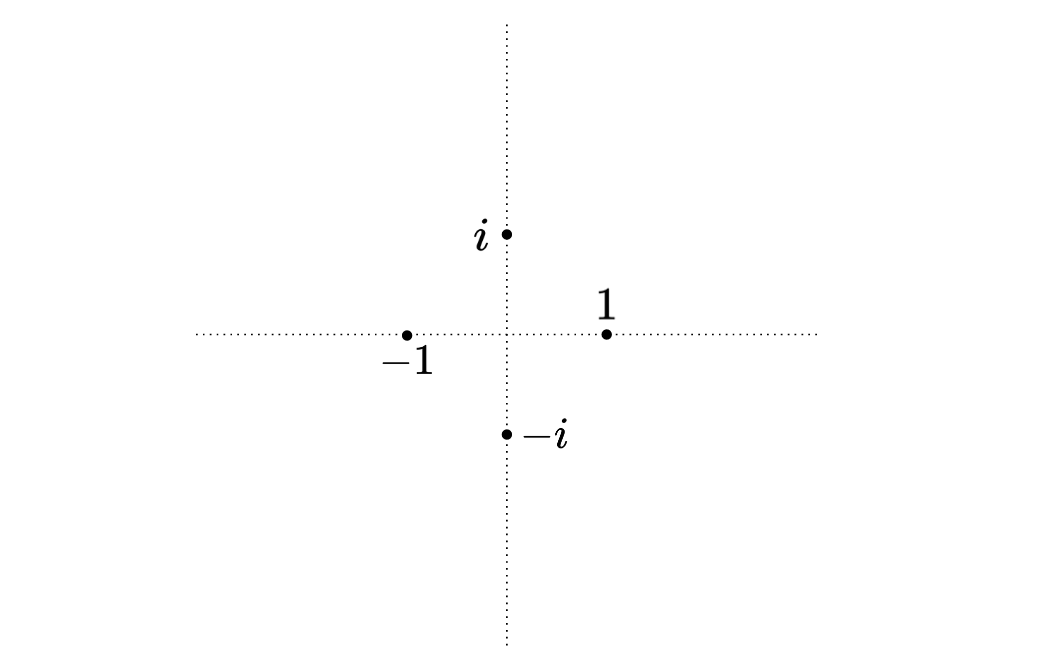
It seems like y multiplying a number with \(-1\) you rotate it by 180 degrees, but by multiplying it with \(i\) you rotate it by 90 degrees.
Fractals
One of them is to draw fractals! Fractals are patterns that repeat forever. If you zoom in what you see is very similar to the whole image. Let's draw a few of them:
Serpinski Triangle
Koch Snowflake
Draw Mandelbrot-Set like a pro!
def is_stable(c, max_iters):
    z = 0
    for i in range(max_iters):
        z = z ** 2 + c
        if abs(z) > 2:
            break
    return i

center_x = -0.1528
center_y = 1.0397
size = 0.000001
max_iters = 100

def color_of(x, y, width, height):
    x = x / width
    y = y / height
    x = (center_x - size / 2) + size * x
    y = (center_y - size / 2) + size * y

    res = is_stable(x + y * 1j, max_iters) / max_iters
    return Color(1, 1, 1) * res
The code allows you to draw arbitrary locations of the Mandelbrot set.
Images as signals
Remember the fourier transform in the previous chapter? There we were trying to inspect which sinusoids exist in a signal. The thing is, we have discovered that the transform can also be applied on images. You can think of a computer image as an array of 1D signals. Applying FFT on rows would tell you exactly how the rows can be decomposed into sinusoids. Here is the magic: you don’t need to stop here, after applying FFT on each row, do it again on each column. The result will help you analyze, how does a signal with a certain frequency varies among rows. An incredible fact is, it doesn't matter if you first apply FFT on rows and the columns are the opposite, the result will be the same. That's probably a good reason why "two-dimensional" FFT is really a solid concept, and not just the result of applying FFT on rows and the columns!
Since FFTs are revertible, you can get the image back from its transformed version by applying inverse-FFT first on columns and then on the rows (Or the opposite, doesn't matter).
We learnt how do fft and ifft work in the previous chapter. We can build two-dimensional fft2 and ifft2 using them like this:
from copy import deepcopy


def fft2(x, inv=False):
    res = deepcopy(x) # Better take a deepcopy to avoid overwrites

    func = ifft if inv else fft

    # FFT on rows
    for i in range(len(x)):
        res[i] = func(res[i])

    # FFT on columns
    for i in range(len(x)):
        col = [res[j][i] for j in range(len(x))]
        fft_col = func(col)
        for j in range(len(x)):
            res[j][i] = fft_col[j]

    return res

def ifft2(x):
    return fft2(x, True)
You can transform a picture to a 2D frequency specturm using the fft2 function, and reconstruct it back using the ifft2 function. Why does this matter? Well, it gives us another perspective on how we can manipulate images. Instead of directly manipulating the pixels of an image, you can first transform it to another "representaiton", change that instead, and then reconstruct it back using the manipulated representation!
Just like audio, generally, the low-frequency components of a signal have greater impact on the signal and by removing high-frequency components, the signal (Be it audio or image) won't change that much. Given this fact, we can try to remove the high-frequency parts (The central sections) of the FFT of an image and see what happens:
SIZE = 1024
image = ... # A 1024x1024 image
fft_image = fft2(image)

for i in range(200):
    for j in range(SIZE):
        fft_image[SIZE // 2 + i][j] = 0
        fft_image[SIZE // 2 - i][j] = 0
        fft_image[j][SIZE // 2 + i] = 0
        fft_image[j][SIZE // 2 - i] = 0

reconstructed_image = ifft2(fft_image)
If you plot the resulting image, you'll see that the change isn't substantial, although we have literally removed a large chunks of the specturm. The only change is that the quality of the image has degraded a bit. We just discovered a compression algorithm for images!
Gradients
def interpolate(a: Color, b: Color, x: float) -> Color:
    return Color(a.r + (b.r - a.r) * x, a.g + (b.g - a.g) * x, a.b + (b.b - a.b) * x)
Adding the 4th dimension!
Now that you know how computer images are made, generating videos is not going to be much harder! If you have the ffmpeg package installed on your system, you can give it a bunch of PPM files to generate a MP4 video for you:
ffmpeg -framerate 10 -i out%d.ppm -c:v libx264 -crf 25 \
-vf "scale=500:500,format=yuv420p" -movflags +faststart output.mp4
Based on the command above, FFmpeg will look for PPM files named out0.ppm, out1.ppm and etc for you, and will then connect them together as a 10 frame-per-second video with the specified encoding/format. You can change the parameters as you wish.
Ray Tracing
3D computer rendering is probably the most complicated and interesting way a computer can stimulate our vision. Our perception is evolved in a way to understand our 3-dimensional space and world. Being able to generate arbitrary 3D looking images with a computer brings us infinite possibilities. Nowadays people are trying to immerse themselves into virtual worlds by putting computer screens really close to their eyes, which renders photorealistic images. There are many methods and algorithms by which we can 3D computer images, we are going to implement two of the most important ones in this book. One of those methods will give you very photorealistic outputs with high rendering times, while the other method gives you inaccurate outputs but is fast enough to generate images in real-time, making it perfect for 3D games.
Surprisingly (Or obviously for some!), the rendering algorithm that gives you real-looking outputs is much simpler to implement, so let's dive in!
Ray-Tracing, as its name suggests is an algorithm, inspired by the science of physics, that tries to generate 3D scenes by predicting and tracking the way photons move in imaginary 3D environements. Since there are infinite number of photons coming out of a light source, it might seem infeasible to generate images with this method. But the fact is, most of the photons coming out of a light source end up somewere that do not have any impact on out final image (They do not reach our imaginary eyes). We only care about those photons that reach our virtual eye/camera. Given this fact we can get clever and do this simulation in a much more efficient way! We just need to go backwards. We will generate rays from our virtual eye and see if they will end up on a lit source! This is the core idea behind the Ray-Tracing algorithm!
The Ray-Tracing algorithm for generating 3D computer images is all about tracing the route a photon goes through when reaching our eyes. You can assume that photons are like particles that are emitted from light sources, as if a lamp is shooting out a lot of ultra tiny balls. These balls change their colors when they hit objects and absorb their colors, and finally some of them reach our eyes, letting us to see the world around us. Since photons move on straight lines, we can study their behavior with mathematical vectors. Since we live in a 3D world, the movements of our photons can be analyzed using 3D vectors. A 3D vector is nothing but a tuple of 3 floating-point numbers. A 3D vector can be used for storing the position or direction of a photon.
class Vec3D:
    def __init__(self, x, y, z):
        self.x = x
        self.y = y
        self.z = z
The most basic operations that can be performed on two vectors is addition and subtraction. We can implement them by overriding the __add__ and __sub__ magic methods:
class Vec3D:
    # ...

    def __add__(self, other):
        return Vec(self.x + other.x, self.y + other.y, self.z + other.z)

    def __neg__(self):
        return Vec(-self.x, -self.y, -self.z)

    def __sub__(self, other):
        return self + (-other)
Besides addition/subtraction, there are two very special and interesting operations that can be done on 3D vectors:
-
Dot-product: Calculates how aligned the vectors are. The dot-product of two vectors is in its maximum when both vectors are pointing at the same direction. The dot-product of two vectors is a scalar value, which can be calculated in two ways:
- \(\vec{A}.\vec{B} = A_x.B_x + A_y.B_y + A_z.B_z\)
- \(\vec{A}.\vec{B} = |\vec{A}|.|\vec{B}|.sin(\theta)\)
-
Cross-product: Calculates how perpendicular two vectors are. The length of cross-product of two vectors is in its maximum when the vectors are perpendicular with each other. The result of a cross-product is a vector, that is perpendicular to both vectors, and its length is equal with the product of length of the vectors multiplied with cosine of their angle. Assuming the cross-product of \(\vec{A}\) and \(\vec{B}\) is \(\vec{C}\), the elements of \(\vec{C}\) can can be calculated with the following formula:
- \(C_x = A_y.B_z - A_z.B_y\)
- \(C_y = A_z.B_x - A_x.B_z\)
- \(C_z = A_x.B_y - A_y.B_x\)
Alternatively, you can calculate the length of a cross-product using this formula:
- \(|\vec{C}| = |\vec{A}|.|\vec{B}|.cos(\theta)\)
Let's go ahead and implement these operations as methods on our Vec class:
class Vec3D:
    # ...

    def dot(self, other):
        return self.x * other.x + self.y * other.y + self.z * other.z

    def cross(self, other):
        return Vec(
            self.y * other.z - self.z * other.y,
            self.z * other.x - self.x * other.z,
            self.x * other.y - self.y * other.x,
        )
Reminding you of high-school math, a 2D vector's length could be calculated by summing the square of vector elements and taking its root, the length of a 3D vector can also be calculated using a similar approach:
\(|\vec{A}|=\sqrt{A_x^2 + A_y^2 + A_z^2}\)
Alternatively, we can calculate the length of a vector by taking the square root of the vector, dotted with itself:
\(|\vec{A}|=\sqrt{\vec{A}.\vec{A}}\)
class Vec3D:
    # ...

    def length(self):
        return math.sqrt(self.dot(self))
Another useful operation is multiplication of a vector by an scalar. We are going to override the
multiplication operator in order to have this operation in our Vec class:
class Vec3D:
    # ...

    def __mul__(self, other):
        return Vec(
            self.x * other,
            self.y * other,
            self.z * other,
        )
Normal of a vector \(\vec{A}\) is defined as a vector with length \(1\) that has the same direction as vector \(\vec{A}\). Based on the definition, we can calculate the normal vector by dividing the elements of the vector by the length of the vector:
\(norm(\vec{A})=\frac{\vec{A}}{|\vec{A}|}\)
class Vec3D:
    # ...

    def norm(self):
        len_inv = 1 / self.length()
        return self * len_inv
Although your compiler's optimizer will do the job for you, it's generally better to calculate the inverse of a number and multiply it with your variables, instead of dividing the variables by a number, since multiplication is a much cheaper operation and will take much less clock cycles of your CPU compared to divisions.
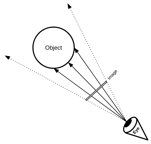
Assuming our imaginary eye is located at \(\vec{E}\), looking at an object that is located on a target \(\vec{T}\), we may assume what is being seen by the eye is reflected on a square plane located with a distance of \(1\), which its center is \(\vec{C}\). Obviously, the direction of \(\vec{EC}\) should be equal with \(\vec{ET}\). Since the size of \(\vec{EC}\) should be 1, we may conclude that \(\vec{EC}\) is the normalized vesion of \(\vec{ET}\).
Now, assuming we have the position of the left-down corner of this plane (\(\vec{LD}\)), and we want to render a \(W \times H\) resolution image, we may loop through each of the pixels on the image and calculate the corresponding 3D point located on the 3D plane (Let's name it \(\vec{P_{ij}}\)), in order to calculate the ray that starts from \(E\)and goes in the direction of \(\vec{EP_{ij}}\).
\(\vec{P_{ij}}=\vec{LD}+\frac{i}{W}\vec{R}+\frac{j}{H}\vec{U}\)
Let's hold the position and direction of a ray in a seperate Ray class:
class Ray:
    def __init__(self, pos, dir):
        self.pos = pos
        self.dir = dir
The rays we are generating are going to propagate through an Environment and hit objects. Let's assume an Environment is made of objects and light-sources. The Environment class is going to have a trace_ray function, which accepts a ray as input, and will return the corresponding color as its output.
class Environment:
    def __init__(self, objs, lights):
        self.objs = objs
        self.lights = lights

    def trace_ray(self, ray: Ray):
        # ...
We can use the PPM image generator we developed in the previous sections in order to calculate a ray-traced scene. We just need to reimplement the color_of function to calculate each pixel according to the environment:
env = Environment([], [])

def color_of(x, y, width, height):
    p = ld + r * (x / width) + u * (y / height)
    direction = (p - e).norm()
    ray = Ray(e, direction)
    return env.trace_ray(ray)
We just saw that we can calculate the initial rays coming out of an imaginary eye if we have the vectors \(\vec{LD}\), \(\vec{U}\) and \(\vec{R}\), but how can we can the vectors themselves?
Assuming our imaginary eye is located at \(vec{E}\) and the target object it is looking at is located at \(vec{T}\), the direction of the eye would be \(norm(\vec{T} - \vec{E})\). Adding this vector to \(\vec{E}\), we'll have a new point that is 1 unit far from the eye vector: \(\vec{C} = \vec{E} + norm(\vec{T} - \vec{E})\)
The vector \(vec{C}\) can be considered as the center of the square plane that we are going to pass our rays through.
Now, remember the definition of cross product: it's a vector that is prependicular to both input vectors. Let's calculate the cross-product of \(vec{EC}\) and a vector that if pointing up \((0,1,0)\) to see what happens. The result will be a vector that is prependicular to both \(vec{EC}\) and the up vector. It'll be pointing to the right of the camera plane (Read about the right-hand rule). The result is \(\vec{R}\). Now calculate the cross-product of \(vec{R}\) with \(vec{EC}\), and you will get another vector that is pointing to the top of the camera plane, it's \(vec{U\})!
Both of the \(vec{R}\) and \(vec{U}\) vectors will be of size 1. In case we want the size of the camera plane's edges to be 1, we can calculate the buttom-left vector as \(vec{LD} = \vec(C) - \frac{\vec{U}}{2} - \frac{\vec{R}}{2}\).
Finally, the resulting camera plane will be a unit square that is 1 unit far from \(\vec{E}\), pointing to target object \(\vec{T}\).
The vectors are visualized in figure X, but it's better to experiment with those vectors yourself and maybe even watch some videos and other ray-tracing tutorials to better get the idea.
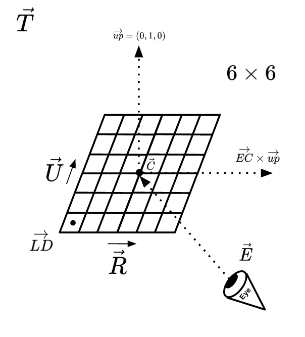
Given the calculations described above, here is the final code calculating everything:
e = Vec(0, 50, 0) # Eye/Camera
t = Vec(0, 0, 100) # Target

ec = (t - e).norm()

c = e + ec # Center of cemera plane
r = ec.cross(Vec(0, 1, 0)) # Pointing to the right of the plane
u = r.cross(ec) # Pointing to the top of the plane
ld = c - r * 0.5 - u * 0.5 # Left-bottom of the plane

def color_of(x, y, width, height):
    p = ld + r * (x / width) + u * (y / height)
    direction = (p - e).norm()
    ray = Ray(e, direction)
    return env.trace_ray(ray)
We are ready to discuss the implementation of the trace_ray function! Let's start with a very simple one: we would like to check if the ray intersects with an sphere. If it does, we would like to return the red color, otherwise black. Since spheres are not the only kind of objects we are going to draw in our ray tracer, it's good to implement things in an object-oriented way already. We'll have an abstract base class Object which will have two abstract functions:
- The
intersectsfunction, will accept aRayand either return an intersection point (As aVec) orNone(If the ray doesn't intersect with the object). color_offunction will accept a point on the object (As aVec) and returns the color of the given point on the object. This allows us to colorize objects.
class Shape:
    def intersects(self, ray: Ray):
        pass

    def color_of(self, pos: Vec):
        pass
class Sphere(Shape):
    def __init__(self, pos: Vec, radius, color):
        self.pos = pos
        self.radius = radius
        self.color = color

    def color_of(self):
        return self.color

    def intersects(self, ray: Ray):
        tca = (self.pos - ray.pos).dot(ray.dir)
        if tca < 0:
            return None
        d2 = (self.pos - ray.pos).dot(self.pos - ray.pos) - tca * tca
        if d2 > self.radius**2:
            return None
        thc = math.sqrt(self.radius**2 - d2)
        ret = min(tca - thc, tca + thc)
        if ret < 0:
            return None
        else:
            return ret
Now we can start seeing the sphere!
sphere = Sphere(Vec(0, 0, 100), 2, (255, 0, 0))

def trace_ray(ray):
    if sphere.intersects(ray):
        return Color(1, 0, 0)
    else:
        return Color(0, 0, 0)
If you render the sphere on a 800x600 image, you'll see that the sphere looks a bit skewed. That's because the imaginary camera-plane we calculated is a unit square, but the aspect ratio of the final image (In this case, 4/3), does not match with the aspect ratio of the camera plane. In order to solve this, you may just apply the ratio difference to the \(vec{R}\) vector:
ASPECT_RATIO = WIDTH / HEIGHT
r = ec.cross(Vec(0, 1, 0)).norm() * ASPECT_RATIO
After this, the sphere should appear like a perfect circle on the image.
The checkerboard plane!
We just rendered an 3D sphere, but the result is not impressive, since it just looks like a 2D circle.
class Checkerboard:
    def __init__(self, normal, intercept, col1, col2, size):
        self.normal = normal
        self.intercept = intercept
        self.col1 = col1
        self.col2 = col2
        self.size = size

    def norm_at(self, pos):
        return self.normal

    def color_of(self, pos):
        if (math.floor(pos.x / self.size) + math.floor(pos.z / self.size)) % 2:
            return self.col1
        else:
            return self.col2

    def intersects(self, ray: Ray):
        div = ray.dir.dot(self.normal)
        if div == 0:  # Plane and ray are parallel!
            return None
        t = -(ray.pos.dot(self.normal) + self.intercept) / div
        if t > 0:
            return t
        else:
            return None
Lighting
After adding the checkerboard plane, you can start to see the 3D-ness of the outputs, but the results are far from being natural yet. The most obvious reason that the outputs look ugly is that we don't have lighting yet. Every point of every object looks as lit as all other points. That's why the sphere we rendered doesn't look much different from a simple 2D circle. In this section, we are going to apply a few types of light-sources to are scenes.
Just like how we abstracted away Shapes, we can also define a base class for every Light we are going to implement like this:
class Light:
    def apply(self, ...)
        # ..
The apply function accepts a few different arguments that may come handy when calculating the light intensity of a point. Since we don't yet know what kind of data may be needed when calculating the light intensity, I put ... instead of the actual arguments. Not all kind of light-sources are going to need all of them. For example, we may have AmbientLights, which will just add a constant color to every point on the scene:
class AmbientLight(Light):
    def __init__(self, col: Color):
        self.col = col

    def apply(self, ...):
        return self.col
Point lights
Point-lights are light-sources that emit light to all directions from a fixed point. Before implementing point light, it's important to understand the Lambertian Reflectance model. The model simply states that: the reflectance of light on a surface is at its highest when the light ray is prependicular to the surface. We can formulate this as if the intensity of light on a point is equal with the cosine of the angle between the normal of that point and the vector looking from that point towards the light-source.
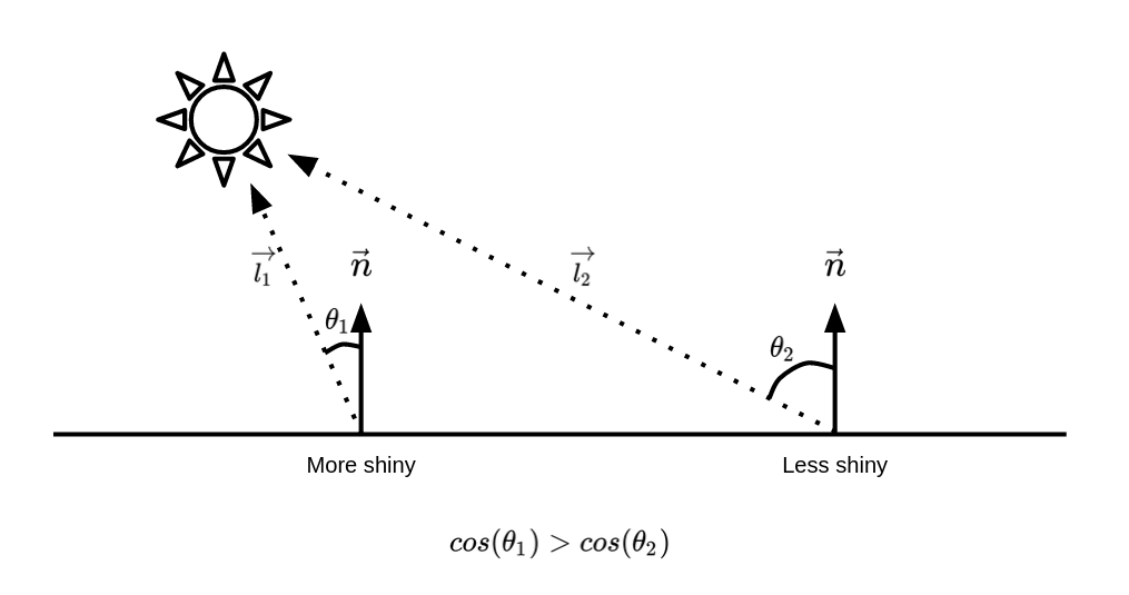
So how do we find \(Since dot-products have the cosine factor in them, we can use them in order to calculate the cosine of the angle between two vectors.
class PointLight:
    def __init__(self, pos: Vec3D, col: Color):
        self.pos = pos
        self.col = col

    def apply(self, env: Environment, ray: Ray, point: Vec3D, norm: Vec3D):
        direction = (self.pos - point).norm()
        intensity = max(norm.dot(direction), 0)
        return self.col * intensity
The power of recursion
What if the photon coming from a point-light is blocked by a secondary object? Then we should have a shadow. Detecting whether there should be a shadow:
class PointLight:
    # ...

    def apply(self, env: Environment, ray: Ray, point: Vec3D, norm: Vec3D):
        intensity = 0
        direction = (self.pos - point).norm()
        ray_to_light = Ray(point + direction * EPSILON, direction)

        # Apply the light only when there isn't any blocking object
        if env.nearest_hit(ray_to_light)[0] is None:
            intensity += max(norm.dot((self.pos - point).norm()), 0)

        return self.col * intensity
class Environment:
    def __init__(self, objs, lights):
        self.objs = objs
        self.lights = lights

    def nearest_hit(self, ray):
        nearest = None
        nearest_dist = float("inf")
        for obj in self.objs:
            dist = obj.intersects(ray)
            if dist:
                if not nearest or (dist < nearest_dist):
                    nearest = obj
                    nearest_dist = dist
        return (nearest, nearest_dist)

    def trace_ray(self, ray, depth=0):
        nearest, nearest_dist = self.nearest_hit(ray)

        if nearest:
            isect_point = ray.pos + ray.dir * nearest_dist
            norm = nearest.norm_at(isect_point)
            l = Color(0, 0, 0)

            for light in self.lights:
                l += light.apply(self, ray, isect_point, norm)

            refl_dir = nearest.norm_at(isect_point).reflect(-ray.dir).norm()

            col = nearest.color_of(isect_point) * l

            if depth < 3:
                refl_col = self.trace_ray(
                    Ray(isect_point + refl_dir * 0.0001, refl_dir), depth=depth + 1
                )
            else:
                refl_col = Color(0, 0, 0)

            return col + refl_col * 0.2
        else:
            return Color(0, 0, 0)
Monte-Carlo method
Although the outputs you are getting from your ray-tracer are already amazing, we can't still claim that they look photo-realistic, and an important reason is that in reality, a photon coming from a light source going to nowhere, may still have some effect
Since we can't take infinite number of photons into account, a solution might simply be to sample a lot of random ones and take an average of them. This is also known as Monte-Carlo method.
Let's explore the Monte-Carlo approximation in a simpler example: approximating the number \(\pi\) by shooting a lot of random points inside a unit square, and counting how many of them are inside the circle. If the random points we are generating are truly uniform, about \(\frac{\pi}{4}\) of them are going to be inside the circle (E.g let's assume we have a square with width \(2\), and a circle with radius 1 inside it. The area of the circle would be \(1^2\pi=\pi\) and the area of the square would be \(2 \times 2=4\), so the circle would be taking \(\frac{\pi}{4}\) of the area of the square)
import random
import math


def is_in_circle(x, y):
    return math.sqrt(x**2 + y**2) <= 1


# Random number between (-1, 1)
def rand():
    return random.random() * 2 - 1


cnt = 0
total = 10000000
for _ in range(total):
    x, y = (rand(), rand())
    if is_in_circle(x, y):
        cnt += 1

print(cnt / total * 4)
This will output a number very close to \(\pi\).
What would the Monte-Carlo approximation mean in the context of ray tracing? Imagine we are calculating the light intensity of a point on a plain. In our current ray-tracer, what we are doing is casting a ray directly from that point to the light source, but in the Monte-Carlo version, we will be casting a lot of rays in different directions and counting all direct/indirect contributions of a light source to that point.
Beyond spheres
- Triangle meshes
- BVH
Rasterization
Rasterization is another effective technique in rendering 3D scenes and it is quite faster than ray-tracing (Or any other method involving simulation of Physics). Although the results are less accurate, it is the main technique used in real-time rendering applications (E.g Video games). You don't have much time to render the next frame in a game! (Although, games are slowly switching to ray-tracing in some parts nowadays, as our hardware becomes faster)
In the rasterization algorithm, instead of emitting rays abd finding the object that it intersects with and calculating its color, we will try to map the 3D points of an object into 2D points on your computer screen through mathematical formula. In other words, when rendering each frame, we loop through the objects in our scene, and all of the 3D points that make those objects, and we will apply a function which convert a triplet \((x, y, z)\) to a pair of floats \((x,y)\). We then fill those pixels on the screen!
Since it is impractical to represent a 3D object by its points (A 3D object it made of infinite number of points), we usually represent them by a bunch of 3D triangles. Looping through the triangles of an object, using the same 3D-to-2D point conversion formula, we can convert a 3D triangle to a 2D one. We just have to apply the function on all three 3D vertices of the triangle in order to get the respective 2D ones.
Filling a 2D triangle on an image is a straightforward process. Before getting into the more complicated parts, let's first draw a triangle on a PPM image, given the 2D position of its vertices. It's good to defined classes for storing 2D points and triangles, so let's first create a class named Vec2D which stores two floating point numbers and another class named Triangle2D for storing three Vec2Ds. Our PPM triangle renderer should accept a Triangle2D and fill the pixels within that triangle.
class Vec2D:
    def __init__(self, x: float, y: float):
        self.x = x
        self.y = y


class Triangle2D:
    def __init__(self, a: Vec2D, b: Vec2D, c: Vec2D):
        self.a = a
        self.b = b
        self.c = c
Matrices, programmable math objects!
When doing ray tracing, we exactly knew where are imaginary eye/camera is, but so far in the rasterization algorithm, we were assuming that the eye/camera is placed at the origin point \((0,0,0)\). So, how could we move in this 3D scene and see it from different perspectives? The solution is a bit different compared to what we were doing in a ray tracer. Here, instead of moving/rotating the camera around the world, we move/rotate all of the objects in that world, in order to make it feel like the camera is placed in a different location! Since we are working with 3D points, before passing the points to the rendering function, we have to apply a transformation function to put the point in a different location.
These transformations are done through matrices! There are matrices that apply certain geometric changes when being multiplicated with vectors.
Assuming our points are represented in 4D vectors where the last element is 1, we can invent a matrix that can move a point by adding a offset vector to it when multiplied with the original vector. This matrix is known as translation matrix. Assuming we want to move our vector \((x, y, z)\) by \((T_x, T_y, T_z)\), the translation matrix works as follows:
\[\begin{bmatrix} 1 && 0 && 0 && T_x \\ 0 && 1 && 0 && T_y \\ 0 && 0 && 1 && T_z \\ 0 && 0 && 0 && 1 \end{bmatrix} \times \begin{bmatrix} x \\ y \\ z \\ 1 \end{bmatrix} = \begin{bmatrix} x + T_x \\ y + T_y \\ z + T_z \\ 1 \end{bmatrix}\]
(We have to add a fourth element in order to make these matrices work)
Nothing explains the concept better than a piece of code. Since all of the transformation matrices we use in this section are 4 by 4 matrices, let's define a Matrix4x4 class for this use and add methods for creating different transformation matrices:
class Matrix4x4:
    def __init__(self, rows):
        self.rows = rows

    @staticmethod
    def translate(offset: Vec3D):
        return Matrix4x4([
            [1, 0, 0, offset.x],
            [0, 1, 0, offset.y],
            [0, 0, 1, offset.z],
            [0, 0, 0, 1]
        ])

    def apply(self, vec: Vec3D):
        # ...
Now, here is an interesting fact about transformation matrices: because of the Associative Property of Multiplication of matrices (\(A \times (B \times C)=(A \times B) \times C\)), they combined with each other, resulting in new 4x4 transformation matrices that behave as if each matrix is applied to the vector independently. This literally means that you can compress infinite number of transformation matrices into a single matrix. As an example, if you multiply two translation matrices which move a point by \((T_{x_1},T_{y_1},T_{z_1})\) and \((T_{x_2},T_{y_2},T_{z_2})\) respectively, you will get a new translation matrix that moves a point by: \((T_{x_1} + T_{x_2},T_{y_1} + T_{y_2},T_{z_1} + T_{z_2})\).
Transformation matrices are not limited to moving points by an offset. There are transformation matrices for rotating objects around different axis too!
\[R_x(\theta) = \begin{bmatrix} 1 && 0 && 0 && 0 \\ 0 && cos(\theta) && -sin(\theta) && 0 \\ 0 && sin(\theta) && cos(\theta) && 0 \\ 0 && 0 && 0 && 1 \end{bmatrix}\]
\[R_y(\theta) = \begin{bmatrix} cos(\theta) && 0 && -sin(\theta) && 0 \\ 0 && 1 && 0 && 0 \\ sin(\theta) && 0 && cos(\theta) && 0 \\ 0 && 0 && 0 && 1 \end{bmatrix}\]
\[R_z(\theta) = \begin{bmatrix} cos(\theta) && -sin(\theta) && 0 && 0 \\ sin(\theta) && cos(\theta) && 0 && 0 \\ 0 && 0 && 1 && 0 \\ 0 && 0 && 0 && 1 \end{bmatrix}\]
Camera matrix
Recall that we move/rotate the world around us instead of placing a camera in an arbitrary position rotation, there is a shortcut way for transforming the world as if a camera at \(\vec{P}\) is looking at a target \(\vec{T}\), and its upper-side is pointing at \(\vec{U}\). This matrix can be created as follows:
\[T = \begin{bmatrix} 1 && 0 && 0 && 0 \\ 0 && 1 && 0 && 0 \\ 0 && 0 && 1 && 0 \\ -P_x && -P_y && -P_z && 1 \end{bmatrix}\]
\(F = normalize(T - P)\)
\(R = normalize(U \times F)\)
\(U = F \times R\)
\[O = \begin{bmatrix} R_x && U_x && F_x && 0 \\ R_y && U_y && F_y && 0 \\ R_z && U_z && F_z && 0 \\ -P_x && -P_y && -P_z && 1 \end{bmatrix}\]
Then the look-at matrix \(L\) can be calculated as follows:
\(L = O \times T\)
The magical matrix
The perspective law says that the distance between 2 points look less when the points get farther of our eyes. There is a magical transformation matrix, called the perspective transformation matrix, which applies this effect for us:
\[\begin{bmatrix} \frac{1}{tan(\frac{FOV}{2})a} && 0 && 0 && 0 \\ 0 && \frac{1}{tan(\frac{FOV}{2})} && 0 && 0 \\ 0 && 0 && \frac{-(Z_{far} + Z_{near})}{Z_{far} - Z_{near}} && \frac{-2 Z_{far} Z_{near}}{Z_{far} - Z_{near}} \\ 0 && 0 && -1 && 0 \end{bmatrix}\]
Where \(FOV\) is field-of-view in radians (Normally \(\frac{\pi}{4}\)), \(a\) is the aspect ratio (Your screen width divided by height), and \(Z_{near}\) and \(Z_{far}\) the closest and farthest objects you can see in the rendered image.
Assuming the output of this multiplication is \((x,y,z,w)\), by dividing the \(x\) and \(y\) components by \(w\), you will get a pair of numbers between \(-1\) and \(1\), which tell you where on the computer screen should this point be rendered. We can map these numbers to points on screen with resolution \(W \times H\):
\(P=(W\frac{\frac{x}{w}+1}{2},H\frac{\frac{y}{w}+1}{2})\)
3D Cube
With the tools we created in the previous sections, we are now able to render a simple 3D cube. Each side of a cube is a square, and therefore consists of two triangles. We will be coloring each side of the cube with a unique color, so that sides are distinguishable with each other.
First, we will need a data structure for storing 3D shapes. Our data structure will be storing the 3D triangles making that object. Let's create a Python class for this purpose and call it Mesh. We will also implement different static-methods generating Mesh objects for different 3D shapes. Let's start with a simple cube-builder:
class Mesh:
    def __init__(self, trigs):
        self.trigs = trigs

    @staticmethod
    def cube(pos: Vec3D, size: Vec3D):
        return Mesh(
            [
                Vec3D(pos.x, pos.y, pos.z), Vec3D(pos.x + size.x, pos.y, pos.z), Vec3D(pos.x, pos.y + size.y, pos.z),
                Vec3D(pos.x + size.x, pos.y, pos.z), Vec3D(pos.x, pos.y + size.y, pos.z), Vec3D(pos.x + size.x, pos.y + size.y, pos.z),
                Vec3D(pos.x, pos.y, pos.z), Vec3D(pos.x + size.x, pos.y, pos.z), Vec3D(pos.x, pos.y + size.y, pos.z + size.z),
                Vec3D(pos.x + size.x, pos.y, pos.z), Vec3D(pos.x, pos.y + size.y, pos.z), Vec3D(pos.x + size.x, pos.y + size.y, pos.z + size.z),
                # TODO
            ]
        )
Barycentric coordinates
In the previous section, we saw how to draw a boring 3D cube with each side filled with a single color. Sometimes you'll want to use an image instead of a plain color on the sides of your object.
Putting image textures on a triangle is a straightforward process: when drawing the 2D triangle, for each of the pixels you are putting on the screen, you must somehow calculate the respective location on an image that the color should be fetched from.
Think!
Music of the chapter: One is glad to be of service - By April Rain
The Game of Life
The Game of Life is a very simple environment and set of rules in which creatures evolve. It was created by the famous mathematician, John Horton Conway to demonstrate, as its name suggests, how a living creature can evolve in a simple environment with simple rules. The model is straightforward. It is a two-dimensional infinite plane of squares, in which each square can be either on or off. Conway's artificial world has 4 rules:
- Any live cell with fewer than two live neighbours dies, as if by underpopulation.
- Any live cell with two or three live neighbours lives on to the next generation.
- Any live cell with more than three live neighbours dies, as if by overpopulation.
- Any dead cell with exactly three live neighbours becomes a live cell, as if by reproduction.
The state of the world in each timestamp in Conway's Game of Life is purely dependent on previous state of the game.
The struggles in building artificial creatures has a long story, but the very first recorded design of a humanoid robot was done in around 1495 by the famous italian polymath, Leonardo Da Vinci.
If you are here to learn about artificial intelligence algorithms, I’m afraid to say you are in the wrong place. We are mostly going to learn about biological inspired algorithms for reaching AGI, because I believe nature has the answers for most of the questions already.
Long story short, interesting things can emerge as a result of many things gathering together, making “complex” system. People have written many books in this matter, in order to amaze you by the fact that intelligence can evolve by connecting many simple things to each other, but here I assume that you are already amazed and want to know how to actually build those stuff?
I would like to remind you the first chapter, where we claimed that interesting things can happen when cause and effect chains of the same type are connected together. That's also the building block of a computer, a lot of logic gates connect together to cause desired behaviors. Interestingly, a human/biological brain is also similar to a logical circuits and digital computers in some ways. A lot of smaller units called neurons are connected together, leading to behaviors we typically call intelligence. There is a huge difference between a digital circuit and a biological brain though. A biological brain is made through the process of evolution, while a digital computer is carefully designed and made by a human, baked on pieces of silicone. When you design a digital computer, you exactly know what you want from it. You want it to make your life easier by running calculations and algorithms that take thousands of years when done by hand. When you do know what you exactly want from something, you can organize it into pieces, where each piece does one and only one independent thing very well, and then connect the solutions of subproblems together, solving the original problem. In case of a digital computer, the subproblems are:
- Storing data -> FlipFlop circuits
- Doing math -> Adder circuits
- Running instructions -> Program Counters
- ...
The fact that the original solution is a combination of solutions of subproblems, means that the solution does not have a symmetric structure. By symmetric, I mean you can't expect the part that solves problem A to be also able to solve problem B. You can't expect a memory-cell to be able to add two numbers. Although they both are logical circuits that accept electrical causes as inputs and produce electrical effects as outputs (And thus they can connect to each other), they have whole entirely different structures.
As humans, it is difficult for us to discover and design decentralized solutions for problems, while it is easy for us to break the problem into subproblems, and find solutions for the subproblems instead.
Interestingly, it's completely the way around for the nature. It's much easier for the nature to design decentralized solutions for the problems, but it's hard for it to break the problem into subproblems, and solve the original problem by solving the subproblems.
Perhaps these are all the reasons why biological brains have very solid, symmetrical structures with complex and magical behaviors and why digital computers are very organized and easy to analyze. I would like to call biological brains and digital computers as dynamic brains and static brains respectively.
Let's define a static brain as a network of gates that are static and do not change their behaviors over time. While a dynamic brain is a network of gates in which the gates themselves can change their behavior and turn into other gates. A static brain is a well organized brain designed by an intelligent creature, in which each part does exactly one thing and cannot change its original behavior when needed (E.g An AND gate cannot change into an OR gate), while a dynamic brain is a network of general-purpose gates evolved by the nature to solve more general problems (E.g. maximizing a goal, like survival, pleasure, etc).
An AND gate inside a computer can only act as an AND gate. It can't change itself to an OR gate when needed. A structure like this may seem boring in the first place, since it can only do one thing and can't change its behavior over time (The neurons/gates in a biological brain can transform, leading to different behaviors). But we can actually bring some flexibility and ability to learn by adding a separate concept known as a memory, which can contain a program and an state. The static circuit's only ability is to fetch an instruction from the memory, and change the state of the system from A to B, per clock cycle. The system's ability to learn comes from it's ability to store an state.
In a dynamic brain on the other hand, the learning can happen inside the connections. There isn't a separate module known as memory in a dynamic brain, but the learning happens when the connections between the neurons and the neurons themselves transform. If we are trying to build an artificial general intelligence, it might make more sense to try to mimick the brain instead of trying to fake intelligence by putting conditional codes that we ourselves have designed.
Unfortunately, we are not technologically advanced enough to build dynamic brains, but we can emulate a dynamic brain inside an algorithm that can run on a static brain. The dynamic gates will be imaginary entities inside a digital memory that can trigger other imaginary gates.
Tunable gates
In order to have a solid and symmetric brain, which is able to learn without losing its uniform shape, we'll need cause/effect gates that are general purpose and can change their behavior.
We can model and-gate as a continuous function on floating point values! We can design a function such that returns 0 by default and approaches 1 only when both its input value are close to 1.
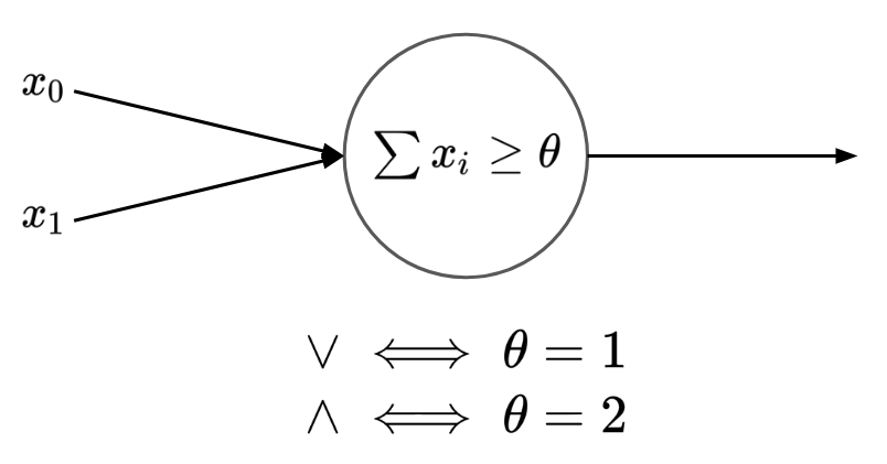
Why modelling a gate as a floating point function is beneficial for us? Because we can take derivative of a continuous function!
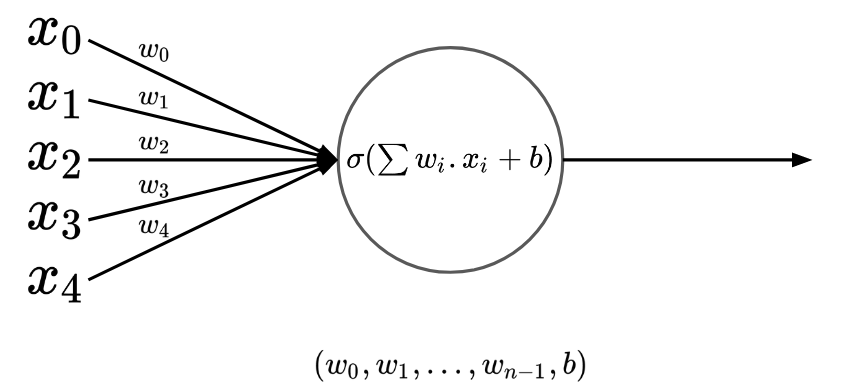
Once upon a time, two nobel prize winners were studying brain cells 1873
Myserious black boxes
Neural networks seem to be blackboxes that can learn anything. It has been proven that they can see, understand or even reason about stuff. Neural Network are known to be universal function approximators. Given some samples of inputs/outputs of a function, neural networks may learn that function and try to predict correct outputs, given new inputs, inputs they have never seen before.
Before feeding a neural network your input data, you have to convert it into numbers. You can encode them anyway you want, and then feed them to a neural network (Which will give you some other numbers), and you may again iterpret the numbers anyway you want, and you can make the network "learn" the way you encode/decode data and try to predict correct outputs given inputs.
Some example encodings:
- Given the location, area and age of a house, predict its price
There are many ways you can encode a location into numbers:
- Convert it to two floating point numbers, longitude and latitude.
- Assume there are \(n\) number of locations, feed the location as a \(n\) dimensional tuple, where \(i\)th elements shows how close the actual location is to the predefined locaiton.
The area/age could also be fed:
- Directly as a number in \(mm^2\) or years
- Interpolated between 0 to 1 (By calculating \(\frac{area}{area_{max}}\))
And just like the way we design an encoding for the inputs, we may also design a decoding algorithm for our output. After that, the neural network itself will find a mapping between input/output data based on the way we encode/decode our data.
Now, one of the most important challenges in designing neural networks that actually work, is to find a good encode/decode strategy for our data. If you encode/decode your data poorly, the network may never learn the function, no matter how big or powerful it is. For example, in case of location, it's much easier for a neural network to learn the location of a house given a longitude/latitude!
A learning algorithm made by humans
Before getting into the details of backpropagation algorithm, let's discuss the mathematical foundations of it first. If you have made it this far in this book without skipping any chapters, you are already familiar with "derivatives", the code idea Newton used to invent his own perception of Physics and motion. Derivative of a function is basically a new function that gives you out the rate of change of the original function on any given point.
The formal definition of derivative is something like this:
\(\lim_{\epsilon \to 0}\frac{f(x+\epsilon)-f(x)}{\epsilon}\)
The "limit" part of the definition means that \(\epsilon\) must be a very small value. Based on this definition, we can numerically estimate the derivative of any function using this piece of Python:
def f(x):
    return x * x

def deriv(f):
    eps = 1e-5
    def f_prime(x):
        return (f(x + eps) - f(x)) / eps
    return f_prime

f_prime = deriv(f)

print(f_prime(5))
Here, the deriv function accepts a single-parameter function and returns a new function that is its derivative (Based on the definition of derivative). The smaller the eps constant becomes, the more accurate our calculated derivatives will get. It's interesting that making eps hugely smaller doesn't make significant difference in the result of the derived function, and will only make it converge to a fixed value. In the given example, the result of f_prime(5) will get closer and closer to 10 as we make eps smaller.
Now, that's not the only way to take the derivative of a function! If you try different xs on f_prime, you'll soon figure out that f_prime is almost exactly equal with x * 2. If we are sure that this is true for all xs, we can define a shortcut version of f_prime function, and avoid dealing with epsilons and fat calculations. That's a great optimization!
You can actually find out this shortcut function by substituting \(f(x)\) in the formal definition of derivative with the actual function. In case of \(f(x) = x^2\):
\(\lim_{\epsilon \to 0}\frac{(x+\epsilon)^2-x^2}{\epsilon}=\frac{x^2+2x\epsilon+\epsilon^2-x^2}{\epsilon}=\frac{2x\epsilon + \epsilon^2}{\epsilon} = 2x + \epsilon = 2x\)
Now, let's imagine we have a set of different primitive functions (Functions that we know their derivatives)
\(\frac{df(g(x))}{dx} = \frac{df(g(x))}{dg(x)} \times \frac{dg(x)}{dx}\)
\(fog(x) = f'(g(x)) * g'(x)\)
def f(x):
    return x * x

def g(x):
    return 1 / x

def fog(x):
    return f(g(x))

fog_prime = deriv(fog)
print(fog_prime(5))

f_prime = deriv(f)
g_prime = deriv(g)
print(g_prime(5) * f_prime(g(5)))
Derivative of the tunable gate
Remember our design of a tunable gate? We can formulate it using a math function:
def f(x, y, b):
    if x + y > b:
        return 1
    else:
        return 0
def sigmoid(x):
    return 1 / (1 + math.exp(-x))
def f(x, y, b):
    return sigmoid(x + y - b)
World's tiniest gradient engine!
I would like to dedicate a section explaining Andrej Karpathy's Micrograd, an ultra-simple gradient engine he designed from scratch which is theoritically enough for training any kind of neural network. His engine is nothing more than a single class named Value, which not only stores a value, but also keeps track of how that value is calculated (The operation and the operands). Here is the full code:
class Value:
    """ stores a single scalar value and its gradient """

    def __init__(self, data, _children=(), _op=''):
        self.data = data
        self.grad = 0
        # internal variables used for autograd graph construction
        self._backward = lambda: None
        self._prev = set(_children)
        self._op = _op # the op that produced this node, for graphviz / debugging / etc

    def __add__(self, other):
        other = other if isinstance(other, Value) else Value(other)
        out = Value(self.data + other.data, (self, other), '+')

        def _backward():
            self.grad += out.grad
            other.grad += out.grad
        out._backward = _backward

        return out

    def __mul__(self, other):
        other = other if isinstance(other, Value) else Value(other)
        out = Value(self.data * other.data, (self, other), '*')

        def _backward():
            self.grad += other.data * out.grad
            other.grad += self.data * out.grad
        out._backward = _backward

        return out

    def __pow__(self, other):
        assert isinstance(other, (int, float)), "only supporting int/float powers for now"
        out = Value(self.data**other, (self,), f'**{other}')

        def _backward():
            self.grad += (other * self.data**(other-1)) * out.grad
        out._backward = _backward

        return out

    def relu(self):
        out = Value(0 if self.data < 0 else self.data, (self,), 'ReLU')

        def _backward():
            self.grad += (out.data > 0) * out.grad
        out._backward = _backward

        return out

    def backward(self):

        # topological order all of the children in the graph
        topo = []
        visited = set()
        def build_topo(v):
            if v not in visited:
                visited.add(v)
                for child in v._prev:
                    build_topo(child)
                topo.append(v)
        build_topo(self)

        # go one variable at a time and apply the chain rule to get its gradient
        self.grad = 1
        for v in reversed(topo):
            v._backward()

    def __neg__(self): # -self
        return self * -1

    def __radd__(self, other): # other + self
        return self + other

    def __sub__(self, other): # self - other
        return self + (-other)

    def __rsub__(self, other): # other - self
        return other + (-self)

    def __rmul__(self, other): # other * self
        return self * other

    def __truediv__(self, other): # self / other
        return self * other**-1

    def __rtruediv__(self, other): # other / self
        return other * self**-1

    def __repr__(self):
        return f"Value(data={self.data}, grad={self.grad})"
Typically, when you have two variables a and b and you add them together in a third variable c, the only thing stored in c is the result of addition of a and b:
a = 5
b = 6
c = a + b
But, let's imagine a world where all values are stored within a Wrapper class, something like this:
a = Wrapper(5)
b = Wrapper(6)
c = a + b
Tensor
If you have had experience doing machine-learning stuff, you know that there is always some tensor processing library involved (Famous examples in Python are Tensorflow and PyTorch). Tensor is a fancy word for a multi-dimensional array, and tensor libraries provide you lots of functions and tools for manipulaing tensors and applying the backpropagation algorithms on them.
Tensor libraries are essential for building super-complicated neural networks. So let's implement a tensor library for ourselves!
A tensor can be simply modeled as a piece of data on your memory which we assume has a particular shape.
As an example, consider the data: [1, 2, 3, 4, 5, 6]. There are multiple ways to interpret these data as multidimensional array:
- 6
[1, 2, 3, 4, 5, 6] - 6x1
[[1], [2], [3], [4], [5], [6]] - 1x6
[[1, 2, 3, 4, 5, 6]] - 3x2
[[1, 2], [3, 4], [5, 6]] - 2x3
[[1, 2, 3], [4, 5, 6]] - 1x2x3x1
[[[[1], [2], [3]], [[4], [5], [6]]]]
See? The data is always the same. It's just the way we interpret it that makes different shapes possible. Given on that, we can implement a tensor as a Python class, holding a list of values as its data, and a tuple of numbers as its shape:
def shape_size(shape):
    res = 1
    for d in shape:
        res *= d
    return res


class Tensor:
    def __init__(self, data, shape):
        if len(data) != shape_size(shape):
            raise Exception()
        self.data = data
        self.shape = shape
We can also make sure that the data and the shape are compatible by checking if data has same number of values as the size of the shape. (You can calculate the size of a shape by multiplying all of its dimension, as we did in shape_size function)
Let's first add some static methods allowing us to generate tensors with constant values:
class Tensor:
    # ...

    @staticmethod
    def const(shape, val):
        return Tensor([val] * shape_size(shape), shape)

    @staticmethod
    def zeros(shape):
        return Tensor.const(shape, 0)

    @staticmethod
    def ones(shape):
        return Tensor.const(shape, 1)
It's also very helpful to print a tensor according to its shape. We do this by first converting the tensor into a regular Python nested-list, and then simply converting it to string:
class Tensor:
    # ...

    def sub_tensors(self):
        sub_tensors = []
        sub_shape = self.shape[1:]
        sub_size = shape_size(sub_shape)
        for i in range(self.shape[0]):
            sub_data = self.data[i * sub_size : (i + 1) * sub_size]
            sub_tensors.append(Tensor(sub_data, sub_shape))
        return sub_tensors

    def to_list(self):
        if self.shape == ():
            return self.data[0]
        else:
            return [sub_tensor.to_list() for sub_tensor in self.sub_tensors()]

    def __str__(self):
        return str(self.to_list())
The sub_tensors function allows us to decompose a tensor into its inner tensors by removing its first dimension. As an example, it can convert a 4x3x2 tensor into a list containing four 3x2 tensors. Having this, we can implement a recursive function to_list which can convert a tensor into a nested-list by recursively converting its sub-tensors to lists.
Mathematical operations in tensor libraries are either element-wise operations that work on scalar values (E.g add/sub/mul/div) or operations that accept two-dimensional tensors (E.g matrix multiplication)
Element-wise operations, as they name suggest, perform the operation on the corresponding elements of two tensors. However, sometimes we can see people adding two tensors with different shapes and sizes with each other. How are those interpreted?
Examples:
3x4x2 + 4x2 = 3x4x24x2 + 3x4x2 = 3x4x25x3x4x2 + 4x2 = 5x3x4x25x3x4x2 + 3x4x2 = 5x3x4x25x1x4x2 + 3x4x2 = 5x3x4x25x1x4x2 + 3x1x2 = 5x3x4x2
Our algorithm:
- Add as many 1s as needed to the tensor with smaller number of dimensions so that the number of dimensions in both of them become equal. E.g. when adding a 5x1x4x2 tensor with a 3x1x2 tensor, we first reshape the second matrix to 1x3x1x2.
- Make sure the corresponding dimensions in both tensors are equal or at least on of them is 1. E.g it's ok to add 5x4x3x2 tensor with a 4x3x2 or a 4x1x2 tensor, but it's NOT ok to add it with a 4x2x2, because \(2 \neq 3\).
- Calculate the final shape by taking the maximum of corresponding dimensions.
This will be the Python code of the mentioned algorithm:
def add_shapes(s1, s2):
    while len(s1) < len(s2):
        s1 = (1,) + s1
    while len(s2) < len(s1):
        s2 = (1,) + s2
    res = []
    for i in range(len(s1)):
        if s1[i] != s2[i] and s1[i] != 1 and s2[i] != 1:
            raise Exception()
        else:
            res.append(max(s1[i], s2[i]))
    return tuple(res)
Now that we have the shape of result tensor, it's time to fill it according to the operation.
Gradient Engines
Our implementation of a tensor is ready, our next big step is now to implement a gradient engine. Don’t get scared by its name, a gradient engine is just a tool you can use to keep track of derivatives of you tensors, with respect to the last computation you perform on your tensors (Which typically shows you how far are the outputs of your network compared to the desired outputs)
Whenever you perform an operation on two tensors, you will get a new tensor. The gradients of tensors a and b is equal with the derivative of the output tensor with respect to each input tensor.
In a production scale neural-network libraries, such as Pytorch and Tensorflow, the building of computation graphs is done automatically. You can go ahead and add tensors and multiply them together using ordinary Python operators (+/-/*). This requires us to implement the magic functions of operators (E.g __add__) in a way such that the resulting tensor keeps track of it parent tensors and is able to change their gradient values when needed. For example, when performing c = a + b, the gradient values of a and b are both influenced by c, so we have to keep track of these relations somewhere. This is done automatically in fancy neural-net libraries. Here we aren't going to make our implementation complicated and prefer to keep our code simple, tolerating some unfriendliness in tensor operations syntax. In our implementation, we assume there is a abstract class named Operator, which all tensor operations inherit from.
from abc import ABC, abstractmethod


class Operator(ABC):
    def __init__(self):
        pass

    @abstractmethod
    def run(self, inps: List[Tensor]) -> Tensor:
        pass

    @abstractmethod
    def grad(self, inps: List[Tensor], out: Tensor) -> List[Tensor]:
        pass
The run function performs the operation on inputs, and then gives us an output tensor. The grad function otherhand, calculates the gradients of inps, given inps and the gradient of the output tensor according to the network's error (out_grad).
Let's take a look at the implementation of the Add operation:
class Add(Operator):
    def __init__(self):
        pass

    def run(self, inps: List[Tensor]) -> Tensor:
        return inps[0] + inps[1]

    def grad(self, inps: List[Tensor], out_grad: Tensor) -> List[Tensor]:
        return [out_grad, out_grad]
The gradient of tensor \(x\) is the derivative of our error function with respect to \(x\).
\(\frac{dE}{dx}\)
It shows us the impact of changing the single tensor \(x\) on the total network error.
Assuming we already know the gradient of the error function with respect to the output of the tensor operation \(\frac{dE}{df(x, y)}\), we can calculate our desired value using the chain operation:
\(\frac{dE}{dx} = \frac{dE}{df(x, y)} \times \frac{df(x, y)}{dx}\)
In case of addition operation, the gradients can be calculated like this
- \(\frac{dE}{dx} = \frac{dE}{df(x, y)} \times \frac{df(x, y)}{dx} = \delta \times \frac{d(x + y)}{dx} = \delta \times 1 = \delta\)
- \(\frac{dE}{dy} = \frac{dE}{df(x, y)} \times \frac{df(x, y)}{dy} = \delta \times \frac{d(x + y)}{dy} = \delta \times 1 = \delta\)
Therefore, the grad function will just return [out_grad, out_grad] as its output!
I assume you already know the way derivation on scalar values work. Derivatives on tensors is also very similar to scalar, the difference is just that, the derivative will also be a tensor instead of an scalar.
Implementing gradient engines is not an easy task at all. A very tiny mistake in calculation of a gradient will invalidate all of the gradient in previous layers. Your neural network will keep training but will never converge to a satisfactory solution, and it’s almost impossible to tell which part of the calculations you did wrong.
There is a very simple debugging idea you can use for checking the correctness of your gradient calculations, which can come handy when developing deep learning libraries. It’s named the gradient check method, and it simply checks if the result of the gradient function is equal with the gradient calculated by hand!
In case of scalar values, the gradient check is something like this:
[TODO]
Language
Large Language Models are perhaps the most important invention of our decade (2020s). LLMs are impressive but they are still using a technology we have known and using for decades, so how we didn't have them before? There are 2 important
- We didn't know a perfect encoding/decoding strategy for text data
- We didn't put enough hardware for training language models
Gate layers
Computation graphs
Different layers
Embedding
An embedding layer is basically a array which you can access its elements. It's often used for converting words/tokens into \(k\)-dimensional vector of numbers. An embedding layer is always put as the first layer in a network, since its inputs are integer indices to elements of a table.
- Propagation:
Y=T[X] - Backpropagation:
dT[X]/dX += delta
As discussed before, sometimes the key to building a good neural network is choosing the way data is encoded/decoded. Since the beginning of the chapter, one of our most important goals was to build a language model. Many of the modern language models are nothing but word-predictors. (Given a list of words, predict the next word). In case of solving the problem using neural-networks, we have to somehow encode the list of words into some numbers that can be feeded to the network, and then interpret the output of the network (Which is a number itself), as a word.
Suppose that the language we are working with is a very simple one and has only 20 words, which are:
I, you, we, they, go, run, walk, say, sing, jump, think, poem, and, or, read, today, now, book, fast, song
Here are some simple sentences in this made-up language:
IrunfastyoureadbookwerunfastandIsingsong
Now the questions is, how can these sentences be feeded to a neural-network which can only perform numerical operations? How do we convert them into numbers?
A very naive encoding for this scenario is one-hot encoding.
One, but hot!
Sometimes, instead of a quantity, you would like to feed a selection among options to a neural-network (E.g a neural network that predicts the longevity of a human given his information. You can clearly see that some of the properties of a human can be quantified, like his/her age, weight and height, but some simply can't). As an example, the gender of a person is not a quantity. In such situations, you can simply assign different numbers to different options and pass those numbers to the network. You can for example assign the number 0.25 for the option man, and number 0.5 for the option woman.
But is this the best way we can encode things to be fed to a network? You will soon figure out that your model will have a very hard time understanding what these numbers mean. That's also the case with real humans. Imagine I tell you property X of person A is 0.25 while for person B is 0.5. You will probably try to interpret those numbers as a quantizable property of a human, but there really isn't a meaningful mapping between a human's gender and his gender. Neural networks are biologically inspired structures, so if it's hard for us to interpret numbers as options, there is a high chance that neural networks can't do it well too.
There is a better way for feeding these kind of information to a neural network, instead of mapping the property to a single number and pass that number through a single neuron to our network, we can have one neuron per option, each specifying the presence of that option in the sample data. In case of our example, assuming we have 2 different genders, we will have two inputs, each input specifying manness and womaness of the data sample.
It's one-hot! One of the inputs is hot (1) and the others are cold (0). It turns our that, networks trained this way perform much better than when the option is encoded as a random, unmeaningfull number. There is also another benefit training a network like this: Imagine a data sample where the man-ness and woman-ness properties are both 0.5. The network will be able to make some sense of it!
Ok, getting back to our example of a language-model, we can use one-hot encodings to encode each word of our sentence as a number. Assuming our model is able to predict the next word of a 10-word sentence, where each word is an option among 20 possible options, our model should accept \(10 \times 20\) numbers as input. That's already a big number. The English language alone has approximately 170k words (According to Oxford English Dictionary), probably without considering many of the slangs and internet words! Imagine having to feed 170k numbers for every word you have in a sentence! This is obviously impractical.
Although one-hot encoding works perfectly when the options are limited, it doesn't work in cases where we have millions of options (E.g a word in a language model). So we have to come up with a different solution.
Let's get back to our dummy solution, where we assigned a number to each word. Let's modify this method a bit: instead of mapping a word to a single number, let's map them to multiple numbers, but in a smart way! Each of the numbers assigned to the words will have a certain meaning. The 1st dimension could specify if the word is a verb or a name, the 2nd dimension could specify if it has a positive or a negative feeling, the 3rd can specify if it's about moving or staying still and so on. This is known as a word-embedding. A mapping between words to \(k\) dimensional numbers. Feeding a a neural networks this way saves a lot of neurons for us. We'll only have to pass \(k\) numbers per each word!
Our language model was getting 10 words as an input and could predict the next word as an output. Imagine we train it and works very well. What will happen if we want to predict the next word of a 3 word sentence? For sure we can’t just put those 3 word on the first three input gates of our network and expect the output to be the fourth word. It is trained to only spit out the 11th word. In fact, the input/ouputs of language models are not like that. A language model of n inputs typically has also n outputs. And each output assumes the input has a certain length:
All you need is attention!
If you have heard of GPT style language models (The most famous one being ChatGPT) the letters GPT stand for Generatice Pretrained Transformer. Here I’m going to talk about a revolutionary neural-network architecture named Transformer, which was first introduced by X scientists in a paper titled: “All you need is attention”
Attention mechanism which has gave us humans the hope that someday we might have AGI, is nothing but a combination of neural-network layers, which happens to be very effective in learning and generating language data.
GPT
GPT is a successfull neural network architecture for language models. It uses the ideas discussed in the Transformer paper. These are the neural network layers used in a GPT:
Assuming the models accepts a sentence of maximum N tokens:
- The model gets
num_tokenstokens as its input. An integer tensor of shape[num_tokens] - The tokens are mapped to
embedding_degree-dimensional numbers, given a lookup-table known as the embedding table. The output of this step is a floating-point tensor of shape[num_tokens, embedding_degree]. - The output of step to goes through
num_layersmulti-head attention layers, where:- For each multi-head attention layers, there are
num_headsheads, wherenum_heads * head_size = embedding_degree- Each head accepts a
[num_tokens, embedding_degree]tensor. - The head is normalized with a LayerNorm function and the result is another
[num_tokens, embedding_degree]tensor. - The k, q and v vectors are calculated by multiplying the input tensor with three different
[embedding_degree, head_size]for that layer. The results are three[num_tokens, head_size]tensors. - k (
[num_tokens, head_size]) is multiplied with q^-1 ([head_size, num_tokens]) giving out a[num_tokens, num_tokens]tensor, telling us how related each word is with other words. - The upper-triangle of the matrix is zeroed out, so that the tokens cannot cheat.
- A softmax layer is applied to convert the importance-matrix into a probability distribution. Now we have a
[num_tokens, num_tokens]vector where sum of each row is 0. - The result is then multiplied with the v vector, allowing the most important tokens to send their "message" to the next attention layers. The output is a
[num_tokens, head_size]tensor.
- Each head accepts a
- Multiple attention-heads with different parameters are applied giving us
num_headsnumber of[num_tokens, head_size]tensors. By putting them besides each other, we'll get a[num_tokens, embedding_degree]tensor. - The
[num_tokens, embedding_degree]tensor is projected into another[num_tokens, embedding_degree]tensor through a linear layer. - The output is added with the previous layer, resulting with another
[num_tokens, embedding_degree]tensor, to kind of give the next layer the opportunity to access the original data and attentioned data at the same time. - The output is normalized. Let's call the result
add_atten_norm. - The output is mapped to a
[num_tokens, 4*embedding_degree]and again mapped to[num_tokens, embedding_degree]through 2 linear layers (This is the somehow the place where "thinking" processes happens). - The output is added to
add_atten_norm, normalized again, and then passed to the next layer.
- For each multi-head attention layers, there are
- The output is normalized.
- The
[num_tokens, embedding_degree]tensor is mapped to a[num_tokens, vocab_size]tensor through a linear layer. - The result is softmaxed, resulting to a
[num_tokens, vocab_size]probability distribution. Each telling you the probability of each token being the next token for each possible sentence-length. (There arenum_tokenspossible sentence-lengths, so we'll havenum_tokensprobability distributions) - Based on the sentence-length, we will decide which row to select, which will give us a
[vocab_size]tensor. We will choose a token among most probable tokens and print it. - We will add the new word to the input, giving us a new input. We will go through the process all over again, getting a new token each time. The text will get completed little by little.
MatMul
Let's say we have \(n\) neurons in a layer, each accepting the outputs of the \(m\) neurons in the previous layer. The neurons in the next layer are each calculating a weighed sum of all the neurons in the previous layer. Looking closely, you can see that the operation is not very different with a simple matrix multiplication!
Matrix multiplication is the most primitive layer used in neural networks. You use a matrix-multiplication layer when you have a layer of neurons where each neuron's input is the weighed sum of all outputs of previous neurons.
- Propagation:
Y=MX - Backpropagation:
dY/dM += XanddY/dX += M
ReLU
ReLU is an activation function to provide non-linearty in a Neural-Network. It's a better alternative for vanilla sigmoid function, since the sigmoid function's closeness to zero can decrease the training speed a lot.
- Propagation:
Y=X if X > 0 else 0 - Backpropagation:
dY/dX += 1 if X > 0 else 0
LayerNorm
LayerNorm is a creative approach for fighting with a problem known as vanishing-gradients. Sometimes when you put plenty of layers in a network, a slight change in the first layers will have enormous impact in the output (Which causes the gradients of the early layers to be very small), or there are times when the early layers have very small impact on the outputs (The gradients will become very high, or explode, in this case). Layer-normalization is a technique by which you can decrease the probability of a vanishing/exploding gradients, by consistently keeping the output-ranges of your layers in a fixed range. This is done by normalizing the data flowing through the layers through a normalization function.
The layer accepts a vector of floating point numbers as input and gives out a vector with same size as output, where the outputs are the standardized version of inputs.
Softmax
Softmax layer is used to convert the outputs of a layer into a probability distribution (Making each output a number between 0 to 1, where sum of all outputs is equal with 1).
\(Y_i = \frac{e^{X_i}}{e^{X_0}+e^{X_1}+\dots+e^{X_{k-1}}}\)
In a softmax layer, each output element depends on the output of all neurons in the previous layer, therefore, the derivative of a softmax layer, is a matrix, so we have to calculate its Jacobian!
Mask
CrossEntropy
CrossEntropy is a strategy for calculating the error of a neural network, where. A CrossEntropy layer accepts a probability distribution as its input, therefore a cross-entropy layer comes after a Softmax layer. In a cross-entropy layer, error is minimized when the output probability of the desired output is 1 and all other outputs are zero. In this scheme, we expect the error of the network to be maximized when the output of the desired neuron is 0, and to be minimized when the output of that neuron is 1. Such behavior can be obtained with a function like \(\frac{1}{x}\) or \(-log(x)\)!
A cross-entropy layer accepts a probability distribution (A bunch of floating point numbers) as input, and produces a single floating point number, representing the error of the network, as its output. The error is defined as:
\(E=-log(X[t])\)
where \(T\) is the index of the desired class. When \(X[t]\) is 0, the error is \(\inf\), and when \(X[t]\) is 1, the error is \(0\). You might first think that we have to consider the outputs of other neurons too, when calculating the error of the network (E.g, we have to somehow increase the error, when the elements other than the one with index \(t\) are not zero, but this is not needed! Assuming that the input to an cross-entropy layer is a probability distribution, forcing the probability of the desired element to become 1, forces the probability of all other non-desired elements to become 0, automatically)
Such a strategy for calculating the error of the network forces the network to learn to select a single option among a set of options. Examples of such use cases are:
- Given a 2D array of pixels, decide if there is a cat, dog, or a human in the picture (An image classifier)
- Given an array of words, decide what word is the next word (A language-model)
Language
Vision
Our path towards Artificial General Intelligence
Here we are going to talk about a philosophical approach of building consciousness in computers.
So we have been doing years and years of research on things so called Artificial Intelligence and Machine Learning, but what I'm talking about here is Artificial General Intelligence, something more than a multilayer regression model used for classifying and prediction. Perhaps the reason we have had a giant progress in development of Machine Learning models is all about money. These things are useful in the world we live in, we can build self-driving cars, smart recommender systems and ... We can't just build a business out of a human-level intelligent system. (Edit: When I wrote this paragraph, LLMs were not as sophisticated as they are today! Things are very different now)
Learning is not enough, genetic matters
You can try teaching Kant Philosophy or General Theory of Relativity to your dog, but I bet it would be disappointing. The mere ability to learn is not enough, the way a brain is wired matters, and that only changes through what we call evolution.
Biological simulation isn't the right path
Although researching on biological side of things could be helpful, but doing it excessively could
We are so close to AGI!
You can hear people saying that our computers can't even simulate the brain of a bee. Humans are smart, nature is dumb, the only thing that is making nature superior than us in engineering self-aware creatures is its vast ability to experiment different random things. Nature can create amazing stuff, but nature is not good at optimizing things. Think of it this way:
The Environment
You want your lovely artificial creature to learn and do amazing things by himself? The first step is to give him the opportunity to do so! How can you expect a chatbot to magically understand the concept of self-awareness without giving it the chance to explore the world and distinguish himself with others? Humans are impressive and amazing, but the environment that was complex (yet not overly complicated) and creative enough that gave organisms the opportunity to evolve to the level of human mind is just brilliant. It's not about how to build a brain, but more about how to build an appropriate environment where a brain can evolve.
Let's act like a God
The very first thing we need for creation of a self-aware creature, is a goal. Simplest form of a goal is survival, which simply means, to exist. In order to make existence a goal, we need to put concepts and things which harms the existence of that creature. We can make the creature dependent on some concept and intentionally take it away from him. Let's call that concept:
Look, but don't touch. Touch, but don't taste. Taste, but don't swallow...
We can't afford infinite randomness
The infinite monkey theorem states that a single monkey randomly hitting the keys of a keyboard for an infinite amount of time can write any given text, even complete works of Shakespear. But our computer resources, as opposed to the atoms in our universe, is limited. So we can't build intelligence by bruteforcing simulated atoms in a simulated world!
Death, gene's weapon for survival
There is no reason for a cell, organism or creature to get old and die, as soon as in some part of its code, it is programmed to restore itself by consuming the materials around him (aka food). But most of the animals die (There are some exceptions, some kind of Marjan in Japan never dies by aging), why that happens? Paradoxically, the death phenomenon can be an important reason why human-level intelligence exists! Only the genes who die after sometime, will survive. The population will boom in an unexpected way and that could lead to the extinction of that specy.
Charles Darwin was always wondering why depression exists.
Consciousness is a loop
There are several evidences supporting the idea, that consciousness is the result of a loop in our nervous system, created during the evolution. Simple creatures do not have it, and the loop gets stronger and stronger when we reach to homo-sapiens. A loop in the input/output gateways of our brain make the "thinking of thinking" phenomenon possible.
People with schizophrenia cannot distinguish between feedback inputs and environmental inputs, so they may hear sounds, that do not exist in real world, driving them crazy. Thinking is like talking without making sounds, and redirecting it back to your brain without hearing it. A healthy brain would expect to hear a sound whenever it talks. Whenever this expectation is somehow broken, the brain cannot recognize if the voice it is hearing is external or it is somebody else inside his brain. It is kind of brain's failure in removing its own voice's echo.
How to experiment self-awareness?
In an experiment known as the "rouge test," mothers wiped a bit of rouge on the noses of their children and placed them in front of a mirror. Before 15 months, children look at the reflection and see a red spot on the nose in the mirror, but they don't realize that the red spot is on their own nose. When children are between 15 and 24 months, they begin to realize that the reflection they see is their own, and they either point to the red nose or try to wipe away the rouge. In other words, they understand that the reflection in the mirror is more than a familiar face–it is their own face.
Last step, abstract thinking
Your creature is now able to find food, escape from dangers, communicate with others and be self-aware. Congratulations! You just built a dog! So what's next? What makes homo-sapiens different with ordinary mammals? People say its our ability to think about things that do not exist. Abstract Thinking isn't a MUST in our world to survive (That's why most animals can't write poems or do math in order to survive), but having it happened to be extremely helpful. Abstract Thinking helped us to unite under the name of
Evolution is decentralized
Humans have always had the dream of replicating themselves by building creatures that have the intellectualual abilities of a human (Or even beyond). You can see how much we fantasize about human-made intelligence in the books, paintings, movies and etc.
Trust!
Music of the chapter: Secret - By The Pierces
I want to tell you a fascination fact about baby humans. Until some age, they can’t distinguish between themselves and others. The concept of “me” is not evolved in their brains, and they might believe in singularity. When they think of something, they are not aware that their mind is isolated from other minds. They think other humans know what they are thinking of. Months pass, and they start to see themselves, as a physical self, in the mirror or by looking at their organs. Babies don’t lie, because they are not aware of concept of lying and the fact that their mind is isolated and they can have “secrets”.
Humans have their own reasons to lie. Evolution has led us to learn lying, and hiding what we know from others. Because perhaps lying is sometimes vital for survival, and those humans who couldn’t lie, couldn’t survive as well. Evolution made us liars, and we should thank nature for that.
Despite its goodness, lying brings distrust. Humans can not build teams and do great stuff without having a solid foundation of trust. You might wonder why evolution has made humans untrustable, when civilization and progress can be made only in a trusted environment? Not completely sure about this, but this is my own personal guess: negative and unethical behaviors are very advanced forms of intelligence. Emergence of bad behavior is the first step of a huge intellectual progress. You can have a big group of animals (Or even stones), who happily live together, because bad behavior has not evolved in them. This might seem nice at first, but it will quickly get boring for the mother nature, because without distrust, there will be no need for more advanced forms of intelligence.
How do you trust someone as a human? The most naive way for us humans to trust other people is to remind ourselves of the history of their interactions with us. We can't read their minds, but we can at least predict and guess how they are going to treat us in the future by analyzing their past behaviors. In order to remember the history of someone, we need to recognize that person. As a human, we normally recognize others by looking at their face (Or hearing their voice, or even their smell).
Humans show different behaviors to different people. They may not talk to an stranger they way talk to their friend, as an example. It is some form of intelligence to show different behavior to different people. Not all of the species are able to to so. A bacteria for example, cannot recognize its sibling bacterias. Bacterias may have a common strategy to behave with other bacterias, either to trust all of them by default, or consider the worst case in its interactions.
Being able to recognize your friend is definitely something that helps the evolution of mind, so it now might seem obvious that why some species have started to be different with each other in terms of looks. Knowing that people recognize, predict and judge others' behaviors by their looks, speeches and the history they have with them, opens a lot of ways to hack it. Knowing all this, people started to take advantage of other people, by putting masks.
This chapter is all about secrets, honesty and trust, and also about facts, dishonesty and distrust.
One of the ingredients of a civilized nation, is the ability to send messages to people, even when they aren't near you. That's why humans invented writing. They started to send messages without speaking, by putting symbols on a piece of paper. That was the start of all of the problems, because now you can't see the face of the writer. How can you know that a message you have received on a letter, is really sent by your friend, or someone that has bad faith (E.g. your enemy)?
Signatures
I would like to define signature as a more general term: a signature is something that is special to someone/something. Your face, your voice, the way you speak, your fingerprint, your handwriting are all examples of signatures. They are special to you, and it's hard to find someone other than you that has the exact same handwriting or face or etc. Therefore, they are an important ingredient of trust. If you know your friend's handwriting well, you can catch a faker/pretender easily, because most probably he can't fake your friend's handwriting very well.
A signature doesn't solve all of the problems. Sometimes you might need to say something to a friend but do not want anybody else to hear it. In a face to face communication, this might be fixed easily (At some level!). You both can go into a private room, and make sure nobody else is nearby. But how can you do this when your message is on a piece of paper, and you don't want to carry the message yourself, but you want a middle man to send it for you. How can you be sure that someone won't read the letter in the middle of the way?
These questions are all discussed and answered in a vast field of science called Cryptography. Cryptography has a long history. Historians claim that the first use of cryptography started sometime around 1900 BC in ancient Egypt. Though the interesting thing is that, the use of cryptographic symbols back then was for people's own amusement (You know, it's fun to break codes and solve riddles). So it was somewhat a kind of art and literature, and not serious attempts in secret communication.
Substitution ciphers were probably the most popular way of coding the messages among ancient people. In a substituion cipher, there is a fixed one-to-one mapping that tells you which character to use instead of a character in the original message. As an example, let's say our mapping simply maps a character to its next character in the English alphabet (This is an example of a Caesar cipher). So the coded version of "hello" would be: "ifmmp". Though this is a very simple mapping and can be easilly hacked (Someone can just try different number of character shifts until something meaningful comes out of the text).
A harder to crack version of a substitution cipher uses random character mappings. This method was sophisticated and seemingly-secure enough that people used it for thousands of years, until an Arab mathematician named Al-Kindi surprisingly showed that it's easy to crack (Sometime around AD 800). He invented a method called frequency analysis. In this method, we first count the number of times each letter happens in large amounts of text (From books and etc), and then build a frequency graph out of it, which shows us which letters are most/least used in the target alphabet. We then do the same thing with the cipher text, and then try to find the mapping with the help of frequency data. As an example, doing frequency analysis on the English alphabet shows us that the E (11.16%), A (8.49%) and R (7.58%) letters are the most widely used characters in English texts, while the Q (0.1962%), J (0.1965%) and Z (0.2722%) are the least used ones. By doing the frequency analysis on the target text (If the encrypted text is large enough!), if we figure out that the letter K is the most common encrypted letter, you can know with a high probability that K is the encoded version of E or A. His discovery is known to be the most important cryptanalytic advance until World War II.
Al-Kindi proposed that we can make frequency analysis methods less effective by using polyalphabetic substititutions. So far we have been describing monoalphabetic substitutions, which means, single characters are encrypted to single character. In a polyalplabetic substitution cipher, multiple letters are substituted with multiple letters. In order to apply frequency analysis attack on a 2-by-2 polyalphabetic substitution cipher, we have to calculate frequencies of aa, ab, ac, .., zx, zy, zz. Analysis gets much harder when the length of mappings is increased.
Discovering the fact that a polyalphabetic substitution cipher is hard to decode (Even with frequency analysis methods), was a huge progress in cryptography. But there is a problem: in order to encrypt and decrypt using n-character to n-character polyalphabetic substitution ciphers, we have to create a unique n-character to n-character mapping, and both the encryptor and decryptor should have a copy of it (Let's call this mapping the secret key). Assuming our target alphabet has \(\alpha\) letters, and we want to substitute \(n\) characters per block, our mapping should have \(\alpha^n\) entries. In case of English language (Without ponctuation marks), we have 26 character. Let's say we would like to use 5-character to 5-character ciphers for encryptions, then our code-book would need to have \(26^5 = 11881376\) entries, which is already a very giant secret key for a very weak encryption/decryption algorithm.
Let's analyze the problem by using more primitive pieces of data as our source texts. Imagine we are working with binary strings. In a binary string, smallest piece of information is stored inside a bit, which can be either 0 or 1. Our alphabet has 2 characters in a binary string so \(\alpha=2\). Now let's say we want to use a monoalphabetic cipher for encrypting/decrypting the string. so we should create a 1-bit to 1-bit mapping for our encryption algorithm. There are only two ways we can build such a mapping!
\(enc_1(0) = 0 \ enc_1(1) = 1\)
And:
\(enc_2(0) = 1 \ enc_2(1) = 0\)
This cipher is very easy to crack. All you have to do as an attacker is to read the cipher text, if it already means something, you have successfully decrypted it, otherwise just swap the bits (I.e change zeros to ones and vice versa), and then, if the source text has some meaningful information and a 1bit-to-1bit encryption algorithm is used, you will get the source text!
So far, we have seen that our secret keys in this scheme have 2 entries. Can we somehow compress this?
Instead of storing the entries for each bit (Which takes 2 bits), we can use a single bit, telling us if we should swap the bits or not!
Let's switch to a polyalphabetic cipher, mapping 2 character to 2 characters each time now. There exist 4 possible substitution mappings now:
\(enc_1(00) = 00 \ enc_1(01) = 01 \ enc_1(10) = 10 \ enc_1(11) = 11\)
Compressed version: \(00\)
\(enc_2(00) = 01 \ enc_2(01) = 00 \ enc_2(10) = 11 \ enc_2(11) = 10\)
Compressed version: \(01\)
\(enc_3(00) = 10 \ enc_3(01) = 11 \ enc_3(10) = 00 \ enc_3(11) = 01\)
Compressed version: \(10\)
\(enc_4(00) = 11 \ enc_4(01) = 10 \ enc_4(10) = 01 \ enc_4(11) = 00\)
Compressed version: \(11\)
Just like how we compressed the 1-char to 1-char mappings into a single bit, we can compress the 4 possible 2-char to 2-char mappings into two bits (Instead of passing all the 4 entries). For each bit of the compressed secret key, we just have to tell if the corresponding bit should be swapped or not.
Definition of secure
The output of an encryption algorithm is known to be secure, when the output binary string looks rubbish, and totally random. Which means, there is no way you can recognize if the output is a string generated by uniformaly picking random letters, or something else.
Some properties of a random string:
- The number of each letter is equal with other letters (In case of a binary string, the number of 1s is equal with 0s)
- ...
XOR is the answer to everything
We can now conclude that, we don't need to store a mapping of size \(2^n\) (\(\alpha=2\) since we are working with binary strings) in order to encrypt/decrypt binary texts. We just need to store a key of size \(n\) bits, which shows us, for each bit, whether we should swap the corresponding bit or not.
Generating the an \(n\) bit key for a n-character to n-character encryption algorithm is as easy as throwing a coin for \(n\) times and fortunately, we all trust the coin flips already!
Although this method can be mathematically proven to be secure (In fact, the method has a name: the one-time padding algorithm), it is not practical, and the reason is that, the keys are not reusable. Suppose we have two messages \(m_1\) and \(m_2\), and a key \(k\) which we’ll use for encrypting both messages:
\(M_1 = m_1 \oplus k\)
\(M_2 = m_2 \oplus k\)
An eavesdropper cannot guess what \(m_1\) is by knowing \(M_1\), but in case he also has a second encrypted message \(M_2\), he can add these two messages together and an something interesting will happen:
\(M_1 \oplus M_2 = m_1 \oplus k \oplus m_2 \oplus k = (m_1 \oplus m_2) + (k \oplus k) = m_1 \oplus m_2\)
If you take the xor of a number with itself, they will cancel-out each other and you will get zero, so the \(k \oplus k\) part is removed from the equation and what you get is basically the sum of messages, which means: \(M_1 \oplus M_2 = m_1 \oplus m_2\), which is definitely a dangerous leak.
To show the importance of the leak, let’s say we want to encrypt two images using this method.
By adding the encrypted images together, you will get a new image which is leaking a lot of information on what the encrypted messages contain.
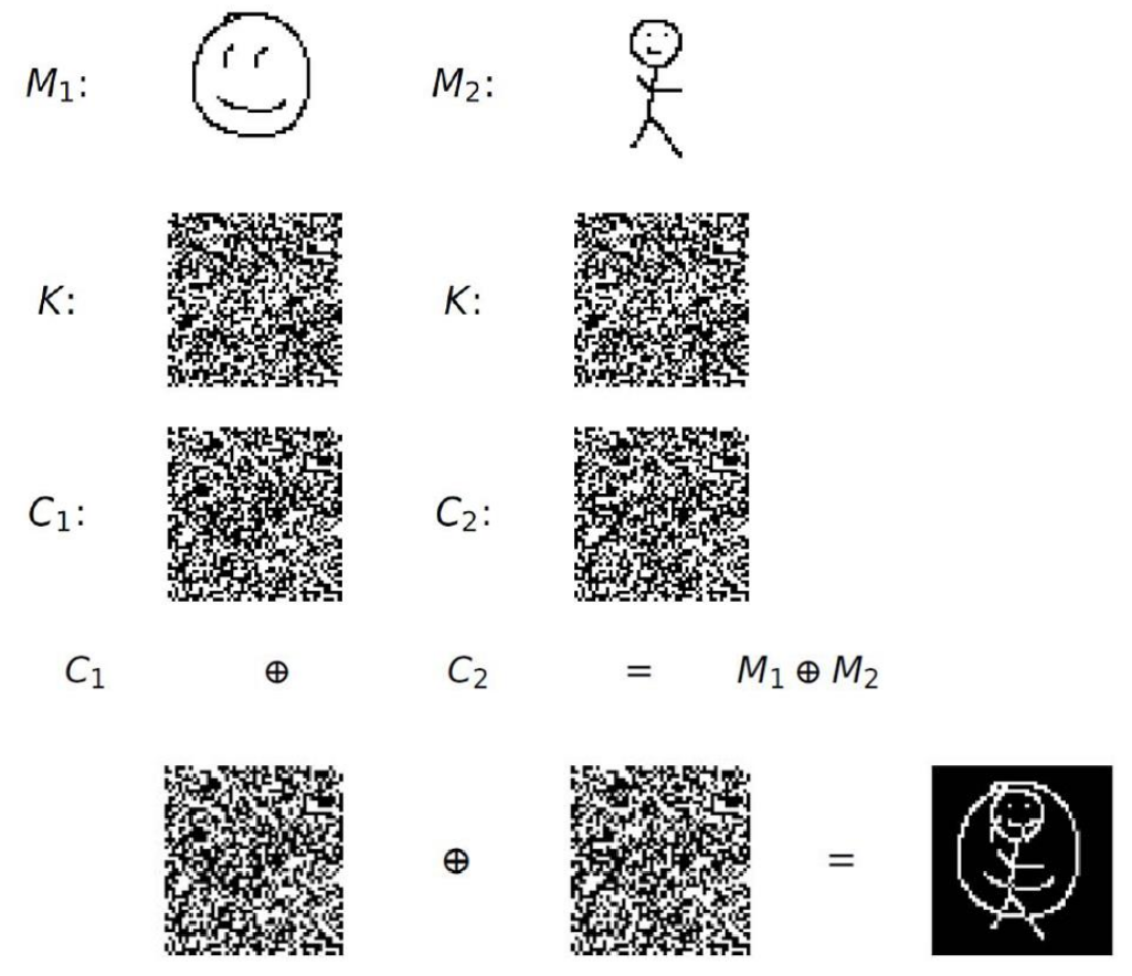
So, the obvious fact here is that, the one-time padding only works if both parties have access to an infinitely large shared random string, otherwise, they will have to exchange a new key every time they want to communicate, and the size of the key should be equal with the size of the message they want to send, which is impractical. In fact, the messages \(M_1\) and \(M_2\) are only obfuscated when the keys used to encrypt them are different:
\(M_1 = m_1 \oplus k_1\)
\(M_2 = m_2 \oplus k_2\)
\(M_1 + M_2 = (m_1 \oplus m_2) \oplus (k_1 \oplus k_1)\)
The summation of two random keys \(k_1\) and \(k_2\) (If both of the keys are totally random and independent with each other), is somehow like a new encryption key \(k_3 = k_1 \oplus k_2\) which has all the randomness properties of \(k_1\) and \(k_2\). This means that \(M_1 + M_2\) will remain encrypted:
\(M_1 + M_2 = (m_1 \oplus m_2) \oplus k_3\)
Unfortunately, our limited computer memory prevents the parties from storing inifinitely large keys, but what if we want to use the provable secure-ness of the one-time padding algorithm, by only having a single key with limited size? There are tricks we can achieve that! A very clever way is to define a function that gets a key \(k\) with a small, fixed-size, and try to expand the binary string to an arbitary length. There are several ways we can do that. A naive method (That just came to my mind while writing this, and has potentially critical security problems!) is to somehow concatenate a pseudo-random binary string to the current string, which is dependent on the current string. An obvious tool for generating such a thing (Based on what we learnt in previous section), is a hash function!
def expand(k, n):
    result = k
    while len(result) < n:
        result += hash(result)
    return result
Signatures
Finite-field elements that we just build are not the only strange kind of group elements besides regular numbers. Matrices exist too, you can define addition and multiplication operations on grids of numbers, and it will behave just as regular numbers.
There is also one very weird kind of group that mathematicians have discovered,
When introducing finite-field, we saw that the algebraic rules that are valid on regular numbers can be valid on other made-up things too! This is not limited to numbers modulo a prime. For example, matrices are also made-up mathematical things that behave very simular to numbers: \((AB)C=A(BC)\) and \(A(B+C)=AB+AC\) and so on.
Making up other things that behave just like regular numbers is fun. One of the most exciting mathematical inventions that ended-up similar to numbers are points that reside on an elliptic curve.
An elliptic-curve is a curve that is defined with a polynomial equation like this:
\(y^2=x^3+\dots\)
For example:
\(y^2=x^3+7\)
By "points", we mean the sets of \((x,y)\) pairs that make the curve equation hold true. E.g, \((1,2\sqrt{2})\) and \((1,-2\sqrt{2})\) are valid points on the curve.
A smart man once assumed that these points are "things" that can be added together, just like numbers. So he had to invent an addition rule that preserves typical rules that apply when working with actual numbers. He had to design the addition rule such that: \((P_1+P_2)+P_3=P_1+(P_2+P_3)\)
Here is what he did: if you pick two points \(P_1\) and \(P_2\), and connect them through a straight line, the line will most probably hit the curve again in an extra point \(P_3\) (Unless the line is completely vertical). Notice that this happens because there is a \(x^3\) component within our equation! If we had a \(x^4\) there, the line could intersect with the curve in two additional points instead of one!
The smart man made an brilliant assumption: if you add points that reside on a straight line together, the result will be some imaginary point that behaves like a zero. So, in case the line intersects with the curve in three points: \(P_1+P_2+P_3=P_{zero}\)
What do I mean by "behaves like a zero"? Just like the regular 0, When you add the zero-point to a point, it should leave it untouched, so: \(P + P_{zero} = P\). For some curves (Like the one we are discussing here) the zero-point does not really exist (I.e you can find a \((x,y)\) pair that acts like a zero-point), so we have to make it up, and pretend it always existed! (Very similar to our approach with imaginary numbers!)
As previously noted, when the line you draw is parallel to the vertical axis, it only intersects with the line in 2 points, which means: \(P_1+P_2=P_zero\). By moving one of the points to the right hand side, we'll get: \(P_2=-P_1\). This means that, you can get the negative of a point by drawing a vertical line passing from that point and finding the intersection.
Also, in the case which the line intersects with 3 points, we can move the third point to the right hand side and then we'll have: \(P_1+P_2=-P_3\). This, together with the method we discovered for finding the negative of a point, gives us a complete method for adding two points. We'll just need to draw a line between the points we are going to add, find the third intersection, and the negate it by finding the mirrored point, as illustrated below:
[IMG]
P = 0xFFFFFFFFFFFFFFFFFFFFFFFFFFFFFFFFFFFFFFFFFFFFFFFFFFFFFFFEFFFFFC2F


def egcd(a, b):
    if a == 0:
        return (b, 0, 1)
    else:
        g, y, x = egcd(b % a, a)
        return (g, x - (b // a) * y, y)


def modinv(a):
    g, x, y = egcd(a, P)
    if g != 1:
        raise Exception("modular inverse does not exist")
    else:
        return x % P


class Point:
    def __init__(self, x, y):
        self.x = x
        self.y = y

    def is_zero(self):
        return (self.x is None) and (self.y is None)

    def is_valid(self):
        return self.is_zero() or (self.y**2) % P == (self.x**3 + 7) % P

    def __neg__(self):
        return Point(self.x, P - self.y)

    def __add__(self, other):
        if self.is_zero():
            return other
        elif other.is_zero():
            return self
        elif self.x == other.x and self.y != other.y:
            return Point(None, None)

        if self.x == other.x and self.y == other.y:
            m = (3 * self.x * self.x) * modinv((2 * self.y) % P)
        else:
            m = (self.y - other.y) * modinv((self.x - other.x) % P)

        x = m * m - self.x - other.x
        return Point(
            x % P,
            (-(self.y + m * (x - self.x))) % P,
        )

    def __str__(self):
        if self.is_zero():
            return "Point(Inf)"
        else:
            return f"Point({self.x}, {self.y})"

    def __repr__(self):
        return str(self)

    def __eq__(self, other):
        return self.x == other.x and self.y == other.y


G = Point(
    0x79BE667EF9DCBBAC55A06295CE870B07029BFCDB2DCE28D959F2815B16F81798,
    0x483ADA7726A3C4655DA4FBFC0E1108A8FD17B448A68554199C47D08FFB10D4B8,
)

print((G + G) + G == G + (G + G))
Electronic Cash revolution
You may already know that I am from Iran, a mysterious country under plenty of sanctions, withholding me from doing any financial activity with people outside our isolated world. We don't have international credit-cards in Iran, and our banking system is completely isolated from the rest of the world (At least when I'm writing this book!). As a young, passionate programmer, spending his teenage years working on "open-source" projects, I was dreaming of getting donations for the work I was publishing online, but I couldn't find any way I could accept money from people on the internet. I couldn't even have something like a PayPal account, it was like a dead-end for me, but you know the end of the story, I found about Bitcoin. I don't remember exactly if I myself looked for an "uncontrollable" (Permissionless?) way of receiving money and found Bitcoin as a result, or a Bitcoin company popped onto my eyes while surfing the internet, anyways, Bitcoin was a saviour for me.
Cryptography was once all about encryption and authentication. It was until recently when mankind started to wonder if he can use computers to build some kind of currency that is not controlled by anyone. Many people might wonder why someone might need something like Bitcoin? Bitcoin helped me, a innocent boy, to escape the limitations I had in my country and transact money with people on the Internet. Bitcoin has been useful for me, and for me, this single usecase is enough to say that Bitcoin is awesome and is already solving problems. If you are a privileged person and have not ever faced problems like this, here might be some reasons why you might need a decentralized currency:
- Privacy - You don't want your government to track every small financial activity you are doing
- Control over your money - You don't want your government to be able to block your money anytime it wants.
- Transaction fees - You don't want to pay excessive transaction fees
- Fault tolerance - You want a payment system that is stable and is available 24/7
We need P2P technologies like Bitcoin to stay safe against governments that are (Or may become) evil (And of course, escape from limitations that are unfair!).
If you read about the history of electronic currencies, you already know that Bitcoin is not the first project that brought the concept on the table. There have been many different attempts by different people to build elecronic payment systems that do not rely on a centralized party. Why they failed and Bitcoin succeeded is that those prior projects were not able to solve a very important problem of such systems, and Bitcoin did. Instead of getting into the details, let's try to model a electronic currency from the ground up, given our limited knowledge, and discover the problem ourselves!
Since you already know some asymmetric cryptography and understand how digital signatures work, let's assume we have a few servers that are connected to each other in a network (Internet perhaps?), and are running the same software. The software is a simple key-value store, mapping public-keys to balances. If a public-key does not exist in the database, we assume the balance of that public-key is 0. Creating an account in such system does not need any interaction, you just need to generate a new private-key in your local machine, and whenever you want to know how much money you have (Which is 0 by default), you will just need to query one of those servers.
Transacting money in such system is as easy as creating a message, in which you clarify who you are (I.e. your public-key), how much and whome you are sending money to (I.e. destination public-key), and then signing the message with your private-key. When those servers receive and read your message, they'll try to validate and process your transaction, and update the balance sheet accordingly.
The transactions also include a unique identifier, so that the servers can recognize if a transatcion is already processed and should not be processed again.
The system works nicely, until someone tries to confuse the network by spending his money twice.
Let's say we have Alice, Bob and Charlie in the network, each having 5 coins according to the balance sheet. Charlie creates two transactions, sending 3 coins to Alice in one, and sending 3 coins to Bob in the other transactions. Obviously, the servers can only process one of those transaction and not both of them, since Charlie doesn't have sufficient fund.
This means the network will have two possible states after hearing those two transactions:
- State #1 Alice: 8 - Bob: 5 - Charlie: 2
- State #2 Alice: 5 - Bob: 8 - Charlie: 2
Charlie can buy a product from both Alice and Bob by sending the same 3 coins to them, effectively spending his coins twice. The problem arises due to the fact that the servers in our network can not agree on the state. Some servers may stop in the #1 state and some in #2, and both states are indeed valid. This problem is known as the Double-Spending problem, and the reason it happens is that the servers can't decide which transaction occurred first.
The classic approach in solving the double-spending problem is to have a central authority deciding the order of transactions. Imagine writing two cheques for Alice and Bob, spending 3 of your coins (While you only have 5). If they go to the bank and try to cash out the cheque at the exact same time, only one of the cheques will pass, since there is a single server somewhere, timestamping the transactions as they happen, disallowing a transaction to happen in case of insufficient balance.
The main innovation behind Bitcoin was its creative solution to the Double-Spending problem, which is called Proof-of-Work. Through Proof-of-Work, the servers in the network could agree only on a single state, without needing a centralized authority. As its inventor describe Bitcoin, Proof-of-Work is a decentralized method for "timestamping" transactions.
The most precious spam-fighter!
Back in 1997, Adam Back, a british cryptographer and cypherpunk, invented something called HashCash. HashCash was a method people could use to fight with denial-of-service attacks (Excessive number of requests trying to get a service down). The idea was to require users to solve a moderately hard puzzle before allowing them to use the service. The solution could also be used as a spam filter (Imagine recipients only accept a mail in their inbox when a solved HashCash puzzle is attached to the mail). HashCash was assuming that we can make the life of attackers/spammers much harder, by requiring them to put significant computation resources for every request/email they make.
The puzzle was to find certain inputs for a hash function such that the output is below a threshold. I can't explain this better than a piece of Python code:
import hashlib


def h(inp):
    return int.from_bytes(hashlib.sha256(inp).digest(), byteorder="little")


MAX_VAL = 2 << 256 - 1
THRESHOLD = MAX_VAL // 10000000

MY_EMAIL = b"Hey, I'm not trying to spam you! :)"

i = 0
while True:
    if h(MY_EMAIL + i.to_bytes(8, "little")) < THRESHOLD:
        print("Nonce:", i)
        break
    i += 1
Imagine a fair dice with 6 sides.
- If you want to get a 1, you must approximately roll the dice for \(\frac{6}{1}=6\) timess.
- If you want to get a \(\leq 2\), you must approximately roll the dice for \(\frac{6}{2}=3\) timess.
- If you want to get a \(\leq 3\), you must approximately roll the dice for \(\frac{6}{3}=2\) timess.
- If you want to get a \(\leq 6\), you must approximately roll the dice for \(\frac{6}{6}=1\) timess.
The same is true with hash functions. Hash functions are analogous to giant dices. As an exmaple the SHA-256 hash function generates outputs between \(0\) to \(2^{256}-1\). In order to get an output below \(\theta\), you will need to try different inputs (Roll the dice) for \(\frac{2^{256}}{\theta}\) times. You can roll a hash-function by "slightly" changing its input (In the HashCash example, we append a small piece of data to the original data and randomly change it until we get our desired output).
In our HashCash example, we require the email sender to "work" approximately as much as running SHA-256 for 1 million times!
Chaining proofs of work!
Satoshi Nakamoto discovered a interesting fact about proof-of-work puzzles. After solving a proof-of-work puzzle, you can append some more data to the whole thing and try to solve the proof of work puzzle again for the new data.
Suppose we first find \(nonce_0\) such that: \(H(data_0 | nonce_0) < \theta\). We then append \(data_1\) to the hash of old data and find \(nonce_1\) such that \(H(H(data_0 | nonce_0) | data_1 | nonce_1) < \theta\)
Solving a proof-of-work puzzle on \(H(data_0 | nonce_0) | data_1\), not only proves that you have worked hard on commiting to \(data_1\), but also shows that you have put equal amount of work to also commit on \(data_0\), for one more time, and that is because altering \(data_0\) not only invalidates the first proof-of-work, but also the second proof-of-work. Assuming that it takes 1 minute to find an appropriate nonce for a piece of data, altering \(data_0\) would invalidate both \(nonce_0\) and \(nonce_1\), meaning that you should find the values for \(nonce_0\) and \(nonce_1\) again, requiring you two solve 2 proof-of-work puzzles, spending two minutes of your CPU time. The longer the chain is, the harder it becomes to alter older data.
Proof-of-Work on financial transactions
Here is the main innovation of Bitcoin: Let's solve proof-of-work puzzles on batches of transactions, and give more priority to those transactions that more work has been done on them! If we apply the chaining trick here too, the older transactions will become harder and harder to be reverted. Let's see and an example in code. We first define two functions which allow us to do proof-of-work on arbitrary pieces of data (aka "blocks")
MAX_VAL = 2 << 256 - 1
THRESHOLD = MAX_VAL // 100000

def is_valid_block(block: bytes):
    return h(block) < THRESHOLD

def mine(block: bytes):
    nonce = 0
    while True:
        if is_valid_block(block + nonce.to_bytes(8, "little")):
            return nonce.to_bytes(8, "little")
        nonce += 1
The is_valid_block function is a criteria for a block to be valid. It simply checks if the hash of the block is below a threshold. In order to make a block's hash below the threshold, we introduce a function which tries adding different "nonce"s to that piece of data and return the nonce that satisfies the condition. Now let's chain some blocks which contain financial data together:
block_1 = "Alice sent Bob 1 BTC, Charlie sent David 2 BTC".encode()
nonce_1 = (88356).to_bytes(8, "little")  # mine(block_1)
block_1_hash = h(block_1 + nonce_1)
if block_1_hash >= THRESHOLD:
    print("Block 1 invalid!")

block_2 = f"Previous hash: {block_1_hash}, David sent Alice 0.5 BTC, Edward sent Charlie 0.2 BTC".encode()
nonce_2 = (275643).to_bytes(8, "little")  # mine(block_2)
block_2_hash = h(block_2 + nonce_2)
if block_2_hash >= THRESHOLD:
    print("Block 2 invalid!")

block_3 = f"Previous hash: {block_2_hash}, Nothing happened!".encode()
nonce_3 = (65352).to_bytes(8, "little")  # mine(block_3)
block_3_hash = h(block_3 + nonce_3)
if block_3_hash >= THRESHOLD:
    print("Block 3 invalid!")
As you can see, block_1 block_2 and block_3 all contain transactions that happen in the network. Practically, those transactions should be structured data which contain real cryptographic signatures, but for simplicity we just assume strings. You can see that I've already found correct nonces and put them in the code for all these three blocks, but finding those takes on average ~100000 hash runs, so it requires computational "work". Now here is the thing: try changing the content of block_2 with something else. E.g, remove the Edward's transaction: block_2 = f"Previous hash: {block_1_hash}, David sent Alice 0.5 BTC".encode(). If you rerun the code, you'll see that not only the block 2 has got invalidated, its subsequent block which is block 3 has also got invalidated! So, in order to change the content within block 2, not only you'll have to run the mine function on block 2, but also on block 3, and that's because the hash of block 2 has appeared in the content of block 3. Now imagine the block "chain" has over thousands of blocks and mining each block requires 1 minute of computation. Changing the block 500 levels behind the tip requires 500 minutes of computational work. So the more blocks are built on top of a block, the harder it gets to change the content of that block.
Now here's what happens in practice: in the actual Bitcoin network, the mining process is actually rewarding. All bitcoin nodes in a network have agreed to consider some Bitcoins for the one who has found the correct nonce for a block. In fact, they allow anyone who builds a "block" to put an extra transaction in the block which says: f"Generate 50 BTC for {miner_address}" and still consider the block valid. So a competetion will happen on generating the blocks, and the competetion is actually so intense that has it actually takes you years of work on a laptop to find correct nonce (The nonce is found in 10-minute timeframe only because there are a LOT of computers over the world who are trying hard to find that nonce), so just imagine how hard would it be to edit the contents of the block 10 levels behind the tip!
There is also one other rule in the network which completes the puzzle. Miner's will give up on working on a block i as soon as someone else finds correct nonce for that block and start working on the next block i+1. So when a block is found, the collective computational power of all bitcoin miners over the world will start working on block i+1, and the collective computational power of those who are still working on block i with a different content will just be so tiny that can't compete with those working on the tip, so it makes more sense for them to give up block i's reward and start working on the tip, so that there is still a chance they could win.
Vanilla KV Stores
Blockchains are one of the coolest types of software you can build from scratch. Implementing one teaches you a lot of things, especially about how data is stored and managed.
One of the most interesting parts of building a Bitcoin-inspired system is handling storage. If you look at Bitcoin Core, you’ll notice it doesn’t rely on traditional databases (SQL or NoSQL). Instead, it mostly uses simple persistent key-value (KV) stores.
Because of that, you need to learn how to safely update the state of the blockchain. Updates should be atomic (they either fully happen or not at all) and reversible (in case you need to roll back a block).
I’ve implemented this kind of system many times out of personal interest, and I’d like to share the model I use for handling it.
Bitcoin as a platform
Bitcoin is safe because the collective computational power of miners working on the bitcoin blocks is so big that people can't revert or edit transactions happening in them.
[MARKER]
Coins with custom locks
Although Bitcoin is the first truly widespread decentralized cryptocurrency, its way of accounting is weird and not so obvious. As a software engineer, You would expect a financial system like bitcoin to have some kind of database that maps addresses to balances, but that’s not the case for Bitcoin. Bitcoin keeps track of its user’s coins through a concept known as UTXOs. Instead of assuming a balance for each bitcoin public key, we keep track of unspent coins with specific Bitcoin value that are tagged with a public key as their owner. These coins can be splitted and merged together, creating new coins with new owners. Remember how Bitcoin considered a reward for those who mine blocks? The miners are those who create the root UTXOs, UTXOs that do not have a parent. There are good reasons why Satoshi decided to do Bitcoin’s accounting this way:
- Avoid spending twice by mistake
- Easier when doing mass transactions
[EXPLAIN BITCOIN SCRIPTS]
Your brand new token hosted by Bitcoin
Bitcoin’s scripting was sufficient for a lot of usecases, but people began to wonder: what if we want to build custom “tokens” that are transferable, just like Bitcoin, but without all those consensus complexities? Do we really need to implement an entirely new Bitcoin software suite from scratch just to create a new coin? That’s not a great idea. What if there are too few users mining our new coin? There must be a smarter way to create new coins without having to worry about double-spending attacks every time.
The answer is simple: instead of viewing Bitcoin purely as a cryptocurrency, think of it as a platform that can host other “tokens” as well. Bitcoin is fundamentally a ledger of balances, so why only store Bitcoin balances in it? Why not allow people to introduce their own coins and store balances for those too? These tokens would automatically inherit all the security guarantees of the underlying currency. If people cannot double-spend Bitcoin, they also won’t be able to double-spend your meme cryptocurrency—even if no one is really using it.
This idea led to the concept of hosting sub-currencies within a currency through a technique known as “colored coins.” Imagine you have 1,000,000 satoshis in your wallet. Now you tell everyone that all the satoshis originating from this particular wallet are also CAT coins. If everyone agrees to treat this as true, those satoshis gain additional value because people handle them differently. Just like that, you’ve introduced a new coin.
Of course, this is not the most robust way to do it.
So Vitalik Buterin thought: why make things complicated? Let’s embed an entire virtual machine (VM) within a blockchain. And that’s how Ethereum was born. A VM is essentially software that simulates an abstract processor with its own instruction set. Vitalik designed the Ethereum Virtual Machine (EVM), which defines instructions that Ethereum nodes can execute.
This instruction set supports typical operations a regular processor can perform—basic arithmetic, loops, and more. In addition to temporary memory, it allows programs deployed on the blockchain to maintain persistent key-value storage, enabling them to keep track of state over time.
Traditionally, a blockchain only tracks balances for each account. Ethereum extends this by allowing each account (specifically, smart contracts) to also maintain its own independent key-value storage, in addition to its balance.
Ethereum introduced the concept of assigning blockchain addresses to programs stored on the blockchain. Just as real users have Ethereum addresses controlled by private keys, Ethereum allows programs to control addresses as well. This means a program can receive ETH just like a user can. The key difference is that when an address controlled by a program receives ETH, its code is automatically executed.
That code determines what happens to the funds. If an exception occurs during execution, the transaction is reverted and the funds are not accepted. Otherwise, the program decides how to handle the money.
Some examples include:
Multisignature wallets Rock-paper-scissors games Scalability solutions Lightning network Plasma cash
Scale
Blockchain transactions are expensive. For every transaction you make, kilobytes of data must be stored not just on one computer, but on thousands of computers around the world (recall that cryptocurrencies are decentralized systems). You can’t simply assume that node runners are willing to sacrifice their precious hard disk space for meaningless data, so they need to “get” something in return for every byte they store.
Even if they don’t receive direct payment for storing your data, the system must at least prevent spam. Otherwise, attackers could flood nodes’ disk space by sending large numbers of tiny transactions across the network. For this reason, transaction fees are a mandatory part of any blockchain system.
Unfortunately, fees are the enemy of scalability. What if I want to make thousands of legitimate microtransactions per second? What if I want to pay a video streamer $0.0001 per millisecond of video I watch? Do I really have to store all those transactions on the blockchain?
That approach would quickly overwhelm blockchains, potentially generating gigabytes of data per second. Clearly, we cannot assume infinite storage or take node runners’ resources for granted.
Even if storage were unlimited, it would still be impossible to validate an enormous number of transactions per second in a decentralized system. However, there are some clever techniques that allow blockchains to scale. I’d like to discuss a few of them—not to turn you into a blockchain engineer, but because these ideas are elegant and interesting, and worth exploring in a book like this.
Let’s start with one of the earliest approaches: Bitcoin’s traditional HTLC (Hashed Time-Locked Contract). Here’s a real-world analogy:
Imagine the blockchain is a bank. You and your friend want to transact frequently, but you don’t want to visit the bank every time you make a small payment and incur a fee. At the same time, you still want the security and enforceability that the bank provides.
Here’s a clever solution:
Suppose you and your friend each deposit $50 into the bank (for a total of $100) and sign a contract stating that $50 belongs to Alice and $50 belongs to Bob. Since both of you have signed it, either of you can present this contract to the bank, which can verify the signatures and distribute the funds accordingly.
Now imagine you both sign a new contract stating that $49 belongs to you and $51 belongs to your friend. This effectively represents you paying your friend $1—but without going to the bank or paying any fees.
These contracts include timestamps, and naturally, the contract with the latest timestamp is considered the valid one. But how does the bank know whether a submitted contract is the most recent? What prevents Alice from submitting an older contract (where she still had $50) and reclaiming money she already paid to Bob?
The solution is this: the bank does not process withdrawals immediately. Instead, it introduces a delay (say, one week) and notifies the other party when a withdrawal request is made.
During this delay, the other party can submit a newer contract if one exists. This proves that the original submitter attempted to cheat by presenting an outdated agreement. As a penalty, the bank can punish the dishonest party—for example, by confiscating their entire balance and awarding it to the other party.
Making Proof-of-Work work less!
Without any doubt, using an incentivized Proof of Work as a way to bring consensus to a public payment network is a revolutionary idea, but there are some obstacles in this method that had been annoying some people, making them wonder if there are any better ideas.
The biggest problem of PoW is its excessive use of energy. Bitcoin (As of 2023) is consuming about 127 TWh per year, and this surely may seem unacceptable by engineers. So people started to play with PoW and try to make it consume less. Part of the reason PoW functions consume a lot of energy is that, people have built specialized hardware for calculating a SHA-256 hash (Known as Application-Specific Integrated Circuit, or ASICs), which is much faster and cheaper than a regular computer, and consumes way more energy. It makes much more sense and profit for people to use these devices instead of wasting their full-featured computers which are designed to do general-purpose computations. So people thought, if we somehow redesign a new hash function, so that building a ASIC for it is almost the same as building a full-featured computer, we may remove the incentive for people to build specialized hardware for it, thus
The earliest ideas in this regard were proposing to make the PoW hash function more dependent on RAM, by requiring a lot of memory to be consumed while generating the hash. Such a hash-function will require a big RAM, and RAMs are surely slow and complicated stuff. Algorithms that do memory operations more often suffer from the memory-access delays. The CPU in this case will be mostly idle, waiting for the memory to return the result. In this case, building a specialized hardware doesn't give you a lot of speed-up, since the memory will be the bottleneck. This makes people to prefer computers over ASICs, leading to overall less usage of energy.
Ready to build a hash function that consumes a lot of memory? Here is a made-up example that is also very inefficient:
import hashlib


def memory_consuming_hash(x):
    farm = [x]
    for i in range(100000):
        farm.append(hashlib.sha256(farm[-1]).digest())
    data = b''.join(reversed(farm))
    return hashlib.sha256(data).digest()


print(memory_consuming_hash(b"123"))
The hash function starts with a list containing the input data. It then goes through a big loop, adding to the list the hash of the last element in the list. Finally, all the items in the list are concatenated with each other and hashed. The reason we are reversing the list before hashing is that, we want to prevent the hasher from simultanously trying to calculate the hash of final input, throwing away the old data (We purposefully want the hasher to memorize everything, otherwise our hash function isn't really memory intensive). If we didn't reverse it, the attacker could simply rewrite the code in a better way so that it requires very small amount of memory.
The proposed hash function is completely made-up, very inefficient and might be insecure. Designing memory-intensive hash functions is a broad topic to discuss, but it explains you the core idea.
Proof-of-Work as a AGI test
I once read someone on X (formerly Twitter) proposing a really interesting test for language models to see whether they’ve achieved AGI-level creativity and intelligence. The idea was to train a model only on data before 2009, before Bitcoin even existed, and then ask it to design a solution for the double-spending problem. If the model independently discovers Proof-of-Work (or some similar mechanism), we could arguably claim that AGI has been achieved! The idea was so clever and compelling that I decided to dedicate a paragraph to it in this book.
Proof of Stake
Bitcoin had an intellectual community back then (It still has!). There were a lot of people talking about ways they can improve Bitcoin in public forums and chat-rooms. One of the revolutionary ideas which was shared as a topic on Bitcointalk was: to expect different hardness of the PoW puzzle from different people, based on their balance. Those with less coins have to work on harder problems, and those with a lot of coins are only required to solve a simple Proof-of-Work puzzle!
If you remember in previous sections, a typical Proof-of-Work puzzle expected you to try, on average, \(\frac{H_{max}}{\theta}\) different nonces in order to find the appropriate nonce. Here we are going to make the puzzle easier for people with more coins. So we somehow have to reduce \(\theta\) in case of a higher stake and reduce it for lower stakes. One way we can handle this is by multiplying \(\theta\) with \(\frac{S_{user}}{S_{total}}\). (Where \(S_{user}\) is this user's stake and \(S_{total}\) is the sum of stakings of all users). This way, the average number of nonce trials needed wiil become \(\frac{H_{max}}{\theta \times \frac{S_{user}}{S_{total}}}\). The higher user's stake is, the closer the fraction becomes to 1, maximizing the possible theta. When the stake of user approaches to zero, the fraction becomes 0 too (Resulting to a smaller theta and a harder puzzle).
The idea discussed above was of the earliest ideas of a Proof-of-Stake consensus algorithm. It really brings in some kind of PoS in the first look but, unfortunately, people with hardware advantages can still take advantage and win all of the blocks. The discussed algorithm is a step towards PoS, but it is not a pure PoS, as it inherits the most weaknesses of a PoW algorithm.
People thought more and more on the nature of a PoS algorithm, and they decided that an ideal PoS algorithm should have nothing to do with a PoW puzzle, but it only has to perform an election between the stakers. The higher you stake, the more chance you will have to win the next block. In order to perform an election in a computer, you will need some source-of-randomness. Let's suppose we have a source of randomness, which gives us values between \(0<r<1\).
Assuming we have \(n\) stakers (Sorted in descending order) \(S_1, S_2, \dots, S_n\), where \(S_T\) is the sum of all staked amounts, we know that \(\frac{S_1}{S_T} + \frac{S_2}{S_T} + \dots + \frac{S_n}{S_T} = 1\). Thus, if we put these stakers on a ribbon, the length of the ribbon will become 1. Now, assuming \(r\) is a random number between 0 and 1, if we mark the corresponding location of \(r\) on the ribbon, it will go inside one of the stakers. We can consider that staker to be the one who is able to generate the next block!
The million dollar question in this method is, who decides the value of \(r\)? Obviously, we can't rely on single party to decide the random number \(r\) for the whole network. The members of the network can not verify if the number provided by the centralized entity is indeed random, or it has purposefully chosen in a way to maximize his own profit.
An interesting method for deciding the random number here is by using a hash function. If you divide the output of a hash function by its maximum value, you will get a floating point number between 0 and 1, which pretty much looks like a uniformly distributed random value. The input given to the hash function can be obtained from the blockchain itself! We can use the hash of last block to get the random value \(r\) used to elect the winner of the next block!
Unfortunately, this method can be easily exploited by an attacker: Imagine the attacker is elected to produce the block \(n\). Now, since the random value of the next block is dependent on the hash of previous block (I.e \(r_{n+1}=h(b_n)\)), the attacker has full control on the value of \(r_{n+1}\). He can alter the block \(b_n\) in a way so that he is elected again for generating the next block! Altering the block can be done in various ways, for example, the attacker can put a dummy transaction in block \(b_n\), sending some funds to himself. The attacker can alter the hash of the block, by simply trying different possible amount values in that transaction. This way, the attacker may win all of the blocks, in case he successfully finds appropriate amount values, making the block have the desired hash value.
Isn't this familiar? That's literally what we were doing in Proof-of-Work! The only difference is that here instead of trying different nonce values, we are trying different amount values in our dummy transaction. The more hardware we have, the higher chance we can win the blocks in the network. We can claim that our proposed PoS algorithm is still a PoW in its heart!
If you look carefully to all these alternative methods, you will see that the source of the problem comes from the fact that the members are able to replay the election process by simply changing some value in previous blocks. If we somehow take this power from the members, and allow the members to generate a random value only once, the problem is solved!
Trust me, it's random!
[TODO]
It's time to commit
Now you probably have an accurate intitution on how cryptographic hash functions work (If you are convinced that the Proof-of-Work algorithm really works). But it's also good to know the formal definition of a cryptographic hash function. A cryptographic hash function is a function that is:
- Collision-resistant: It's hard to find a pair of \(x\) and \(y\) where \(H(x)=H(y)\).
- Preimage-resistant: Given \(y\), it's hard to find \(x\) where \(H(x)=y\).
- Second-perimage-resistant: Given \(H(x_1)=y\), it's hard to find \(x_2\) where \(H(x_2)=y\).
Besides generating proofs of work, there are other interesting things you can do with hash functions. In general, cryptographic hash functions let you to commit to a secret value, and reveal it later.
Cryptographic games
A useful example is when you want to play the Rock/Paper/Scissors with your friend over phone. You can agree to shout out your choice simulatanously, but there is always the chance that your friend may hear your choice and make his choice based on that, always winning the game. What if you guys want to play Rock/Paper/Scissors over physical letters? It'll become much harder to prevent cheatings! Cryptographic hash functions come handy here:
- Alice chooses his option \(a\), but instead of revealing \(a \in {R, P, S}\), she reveals \(H(a)\).
- Just like Alice, Bob chooses \(b \in {R, P, S}\), and reveals \(H(b)\).
- Now both Alice and Bob know that their opponent has made his choice and commited to it, so they can reveal their choices.
- They both will check if their opponent's choice matches with their commited value (If it doesn't, it means the opponent is cheating).
- If everything is alright, winner is determined according to \(a\) and \(b\).
There is a hack to this approach. Since the options are very limited, both Alice and Bob can pre-compute a table of all possible choices and their respective hashes. Then they'll be able to know their opponent's movement based on their commited value. We can prevent this by introducing an extra random value appended to the input of the hash function, known as a salt. (It's dangerous to directly store the passwords of the users in a web-application's database. It's also dangerous to store hashes of the passwords, since many users choose weak passwords and attackers may build pre-computed tables by trying many different popular passwords, just like what an attacker can do in the Rock/Paper/Scissors game we just designed, so you have probably seen that a random salt is added to the user's password before applying the hash function. The salt is stored on the database for later verifications).
It's nice to remember: Whenever you are designing a cryptographic protocol and would like to prevent attacks based on precomputed-tables, adding a salt is a efficient and good solution.
The following Python code will let you to generate commitments for participating in a cryptographic Rock/Paper/Scissors game:
import random, hashlib

choice = input("Choice? (R/P/S)")
assert choice in ["R", "P", "S"]

# Generate a random 16 letter alphanumeric salt
salt = "".join(random.choice("0123456789ABCDEF") for i in range(16))

commit = hashlib.sha256((choice + salt).encode("ascii")).hexdigest()

print("Salt (Reveal it later!):", salt)
print("Commit:", commit)

# Reveal choice and salt later
After both you and your opponent have got the commitments of each other, you may now reveal your choices and respective salts. The following Python3 program may be used for finding the winner:
import hashlib

alice_choice = input("Alice choice? ")
alice_salt = input("Alice salt? ")
alice_commit = input("Alice commitment? ")

if alice_choice not in ["R", "P", "S"]:
    print("Alice has made an invalid move!")

if (
    alice_commit
    != hashlib.sha256((alice_choice + alice_salt).encode("ascii")).hexdigest()
):
    print("Alice is cheating!")

bob_choice = input("Bob choice? ")
bob_salt = input("Bob salt? ")
bob_commit = input("Bob commitment? ")

if bob_choice not in ["R", "P", "S"]:
    print("Bob has made an invalid move!")

if bob_commit != hashlib.sha256((bob_choice + bob_salt).encode("ascii")).hexdigest():
    print("Bob is cheating!")

# Winner may now be determined based on alice_choice and bob_choice!
print("Alice:", alice_choice)
print("Bob:", bob_choice)
Commiting to a set of values
Not only you can commit to a single value, but you can commit to multiple values, and later prove and reveal the existence of a certain value in the set. Here is a silly cryptographic game where commiting to a set of values might be useful. Imagine I have chosen a number between 0 to 1000, and I want you to make 20 guesses on what my number is. You may take 20 random guesses and commit to it by taking the hash of a comma seperated string, containing all of your guesses. You can then reveal your guesses and I can check:
- If you really have only chosen 20 numbers, and not more (Just split the comma-seperated string by
,and check its length) - If your guess list includes my number
Now, there is problem. What if the guess list is very large? (Imagine millions of numbers). You have to reveal all of my guesses, otherwise I can't check if your commitment matches your numbers. Is there any way I can prove existence of a certain number in my list, without revealing all other numbers I have in the list? (Both for privacy and performance reasons). There is!
Binary trees are your best friend, any time you want to optimize the space-efficiency or computation-efficiency of something related to computer science!
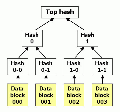
Inventing a new math
The math we are used to, is all about different operations you can perform on numbers. You can add them, subtract them, multiply them or divide them by each other. These operations (If you are not really into math) only make sense if the operands are number. For example, you can't add an apple to an orange, it's meaningless, because the definition of addition is meaningless in case of fruits. But let's assume it's possible, and try to invent some new kind of math for fruits. Imagine the fruits we are working with in our new math are: Apple, Orange and Banana. There are 9 different possibilies when fruits are added together (\(3 \times 3\)), and since the result of adding two fruits is also a fruit, there will be a total of \(3^9\) ways we can invent the \(+\) operation on fruits. Here is an example:
| A | B | A + B |
|---|---|---|
| Apple | Apple | Orange |
| Apple | Orange | Orange |
| Apple | Banana | Apple |
| Orange | Apple | Banana |
| Orange | Orange | Orange |
| Orange | Banana | Banana |
| Banana | Apple | Apple |
| Banana | Orange | Orange |
| Banana | Banana | Banana |
Unfortunately, the math we have just invented on fruits does not obey some of the properties we are used to when adding numbers. For example, you might expect that \(Orange + Banana\) is equal with \(Banana + Orange\), but in our new, randomly invented math, that's not the case. There are other missing features too, for example: \((Apple + Orange) + Banana\) is not equal with \(Apple + (Orange + Banana)\)! Try to redesign the \(+\) operation, so that we have the mentioned properties in our fruit-math too.
Here is an example of a fruit-math that perfectly obeys the mentioned laws:
| A | B | A + B |
|---|---|---|
| Apple | Apple | Apple |
| Apple | Orange | Orange |
| Apple | Banana | Banana |
| Orange | Apple | Orange |
| Orange | Orange | Banana |
| Orange | Banana | Apple |
| Banana | Apple | Banana |
| Banana | Orange | Apple |
| Banana | Banana | Orange |
Let's make our fruit-math more interesting. Addition is not the only operation we can do on numbers. We can do multiplications too. Just like additions, multiplication of fruits is also meaningless (Even more meaningless than addition!), but that's ok, just like what we did with the addition operator, we can also design a table for multiplication. There will be \(3^9\) different possible defintions for \(\times\). If we start with a random table, we will lose some of the properties \(\times\) operator has on regular numbers. In case of regular numbers, we know that \(a \times b\) is equal with \(b \times a\). There is also one very unique and important property that we have on regular numbers. \(a \times (b + c)\) is equal with \(a \times b + a \times c\). Try to design \(\times\) operator on fruits so that it obeys these properties too. You will probably reach to a table like this:
| A | B | A * B |
|---|---|---|
| Apple | Apple | Apple |
| Apple | Orange | Apple |
| Apple | Banana | Apple |
| Orange | Apple | Apple |
| Orange | Orange | Orange |
| Orange | Banana | Banana |
| Banana | Apple | Apple |
| Banana | Orange | Banana |
| Banana | Banana | Orange |
Since there are limited number of addition/multiplication tables that obey math rules we are used to, we can conclude that there are very few varities of math we can design for Apples, Bananas and Oranges. One clever way to easily extract new fruit-maths is to use substitute the fruits in our current tables with another permutation of fruits (E.g. change Apple->Banana, Banana->Orange and Orange->Apple). But who are we going to fool! These tables are still somehow equal with the first table, and we haven't really invented a new math! There is even a scientific word for it, the tables generated this way are actually isomorph with each other, or in other words, there exists a mapping for the elements in the first table, that migrates us to the second table!
Strangely, out of \(3^9.3^9\) possible ways we can invent a math for fruits (Assuming we want to fill the addition and multiplication tables), only few of them are valid and behave as expected, and all of those valid maths are isomorph with each other, meaning that effectively, we only have a single kind of math, in case we have 3 number of elements! Mathematicians refer these kind of maths as: Finite-fields
Now imagine we use substitute Apples, Oranges and Bananas with numbers under 3 (0, 1, 2), respectively (Obviously, we will get an isomorph). Here is how the addition and multiplication tables will look like:
| A | B | A + B |
|---|---|---|
| 0 | 0 | 0 |
| 0 | 1 | 1 |
| 0 | 2 | 2 |
| 1 | 0 | 1 |
| 1 | 1 | 2 |
| 1 | 2 | 0 |
| 2 | 0 | 2 |
| 2 | 1 | 0 |
| 2 | 2 | 1 |
| A | B | A * B |
|---|---|---|
| 0 | 0 | 0 |
| 0 | 1 | 0 |
| 0 | 2 | 0 |
| 1 | 0 | 0 |
| 1 | 1 | 1 |
| 1 | 2 | 2 |
| 2 | 0 | 0 |
| 2 | 1 | 2 |
| 2 | 2 | 1 |
Strangely, we can see that the addition/multiplication tables are basically just modular addition/multiplication! (I.e addition and multiplication modulo 3).
Making things hard
Now, let's discuss one of the most fundamental assumptions that made modern cryptography possible. I would like to start with a simple equation. Find \(x\) such that:
\(3^x = 243\)
Finding the correct value of \(x\) in such an equation is not going to be difficult. You'll just need to take the logarithm of the right hand side of the equation, and you'll have the correct \(x\). You'll basically divide the right hand side by \(3\), until it gets \(1\). \(x\) is the number of times you have done the division.
Let's change the equation a little bit, by switching to a made-up mathematics (E.g mathematics defined on numbers modulo 19) that we discussed earlier! Here is the new equation, try to solve it:
\(3^x \mod 19 = 4\)
Unfortunately, this equation is not as simple to solve as the previous one. We discussed how addition and multiplication can be done on our made-up math, but we didn't discuss how we can divide two numbers! So, our best bet is to try to brute-force the problem, by trying all different \(x\)s:
- \(3^0 \mod 19 = 1\)
- \(3^1 \mod 19 = 3\)
- \(3^2 \mod 19 = 9\)
- \(3^3 \mod 19 = 8\)
- \(3^4 \mod 19 = 5\)
- \(3^5 \mod 19 = 15\)
- \(3^6 \mod 19 = 7\)
- \(3^7 \mod 19 = 2\)
- \(3^8 \mod 19 = 6\)
- \(3^9 \mod 19 = 18\)
- \(3^{10} \mod 19 = 16\)
- \(3^{11} \mod 19 = 10\)
- \(3^{12} \mod 19 = 11\)
- \(3^{13} \mod 19 = 14\)
- \(3^{14} \mod 19 = 4\)
Voila! The solution is \(x=14\)! Let's not stop here and keep trying higher \(x\)s:
- \(3^{15} \mod 19 = 12\)
- \(3^{16} \mod 19 = 17\)
- \(3^{17} \mod 19 = 13\)
- \(3^{18} \mod 19 = 1\)
- \(3^{19} \mod 19 = 3\)
- \(3^{20} \mod 19 = 9\)
- \(3^{21} \mod 19 = 8\)
- \(\dots\)
After \(3^{18}\), we'll see that the results are repeating again. It looks like a cycle! In fact, you can start with any number under 19, after multiplying it by 3 for 18 times, you'll get back to that number again!
\(a \times 3^{18} \mod 19 = a\)
Let's try a different modulus this time. For example, let's try 23. This time, you'll see that the cycle happens after 22 iterations. It seems like that:
\(3^{m-1} \mod m = 1\)
But that is not the case! Try 25:
- \(3^{0} \mod 25 = 1\)
- \(3^{1} \mod 25 = 3\)
- \(3^{2} \mod 25 = 9\)
- \(3^{3} \mod 25 = 2\)
- \(3^{4} \mod 25 = 6\)
- \(3^{5} \mod 25 = 18\)
- \(3^{6} \mod 25 = 4\)
- \(3^{7} \mod 25 = 12\)
- \(3^{8} \mod 25 = 11\)
- \(3^{9} \mod 25 = 8\)
- \(3^{10} \mod 25 = 24\)
- \(3^{11} \mod 25 = 22\)
- \(3^{12} \mod 25 = 16\)
- \(3^{13} \mod 25 = 23\)
- \(3^{14} \mod 25 = 19\)
- \(3^{15} \mod 25 = 7\)
- \(3^{16} \mod 25 = 21\)
- \(3^{17} \mod 25 = 13\)
- \(3^{18} \mod 25 = 14\)
- \(3^{19} \mod 25 = 17\)
- \(3^{20} \mod 25 = 1\)
Our prediction didn't work out, the cycle happened after 20 iterations! In fact, after trying different examples, we'll soon figure that our prediction is true only when the modulus is a prime number! So, how can we predict the cycle length in case of a non-prime modulus?
Swiss mathematician, Leonhard Euler, designed a formula for that purpose in 1763. It's also known as Euler's totient function, and is defined as below:
\(\varphi (m)=p_{1}^{k_{1}-1}(p_{1}{-}1),p_{2}^{k_{2}-1}(p_{2}{-}1)\cdots p_{r}^{k_{r}-1}(p_{r}{-}1)\)
(Assuming \(m=p_1^{k_1}p_2^{k_2}p_3^{k_3} \cdots p_r^{k_r}\))
He also stated, in the Euler's theorem, that:
\(a^{\varphi(m)} \equiv 1 {\pmod {m}}\)
So, in the previous example, we know that \(25=5^2\), therefore, \(\varphi(25)=5^{2-1}(5-1)=20\), so if we start with some random number \(a\) and multiply by itself for 20 times, we'll get back to the original number!
A mathematical private mailbox
Now, using the facts mentioned above, we would like to design a public-key cryptography system. In such cryptographic protocol, one can encrypt a message \(a\) by calculating \(A=a^e\) (Where \(e\) is an encryption key, which is public for everyone), and the receiver can decrypt it by calculating \(a=A^d\).
Let's forget about the generalized form of totient function and only focus on composite numbers of form \(m=pq\). In this case, the output of the totient function is \(\varphi(m)=(p-1)(q-1)\) which means:
\(a^{(p-1)(q-1)} = 1\)
(You might first think that \(e=p-1\) and \(d=q-1\) are practical candidates for \(e\) and \(d\), but they are not, since the right hand side of the equation above is \(1\) instead of \(a\))
Therefore:
\(a^{(p-1)(q-1) + 1} = a\)
We need to find \(e\) \(d\) such that for every \(a\): \((a^e)^d=a\). In fact, \(ed\) should be equal with \((p-1)(q-1)+1\). Finding such numbers isn't too difficult, but we are not going to discuss that.
Now let's say Bob calculate \(e\) and \(d\) gives the number \(e\) to Alice and keeps \(d\) for himself. Let's say Alice has a message \(a\) which wants to send to Bob, but doesn't want anyone but Bob to read it. Instead of \(a\), she can send \(A=a^e\) to Bob. Upon receiving, Bob can calculate \(a=A^d\), and get the original message back.
Diffie-Hellman
We have two people who want to send a physical letter to each other. They can send their letters through a postman (Who unfortunately is very nosy!). They don't want the postman to read the letter. Sender and receiver both have a lock and its key that can put on the box. They can't send their keys to each other! How can the sender send privately send the letter?
- The sender puts the letter in the box and locks it and sends it to the receiver.
- The receiver locks the box with his key too, and sends it back to the sender.
- The sender opens his own lock and sends it back to the receiver.
- The receiver may now open the box and read the letter.
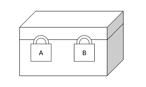
Stealth addresses!
The Diffie-Hellman key-exchange algorithm allows you to calculate a shared-secret between two parties, even when someone is eavesdropping your communication line. Now instead of two people, imagine there are many people participating in a similar scheme, each having their own public-key. Assume on of them wants to send a message to another one in the network, but doesn't want other people in the network to know who he wants to talk with. As a first step, the sender should broadcast his message to everyone, instead of routing it to his desired destination (Because others will know with whom the sender is communicating, even though the messages are all encrypted and private).
- Bob generates a key \(m\) (Master private key), and computes \(M = g^m\) (Master public key), where \(g\) is a commonly-agreed generator point for the elliptic curve.
- Alice generates an ephemeral key \(r\), and publishes the ephemeral public key \(R = g^r\).
- Alice can compute a shared secret \(S = M^r\), and Bob can compute the same shared secret \(S = m^R\) (Very similar to Diffie–Hellman key exchange we just discussed).
- A new public-key can be derived for Bob: \(P = M + g^{hash(S)}\) (Elliptic-curve point addition).
- Bob (and Bob alone, since he only knows the value of \(m\)) can compute corresponding private-key \(p = m + hash(S)\) (Scalar addition).
Now, the receiver may listen to all ephemeral points broadcasted in the network and will try to see if any message is being sent to the corresponding derived public-keys, and see if someone was meaning to communicate with him. In this scheme, only the receiver is able to know that someone is communicating with him, and not anyone else.
[TODO]
Do my computation!
I have always been very curious about different ways we can write programs. Object Oriented, Functional, imperative and etc, all require different kinds of thinking, and it was always exciting for me to learn new languages that introduces a new kind of thinking. Years I have been out of languages that were truly introducing a conpletely new concept, but R1CS is one of the most interesting ways you can program stuff.
R1CS doesn’t actually give you a set of instructions to write your program with, it is not a language at all. It’s a way you can force someone to perform the computation you desire, by solving math equations.
R1CS, short for Rank-1 Constraint System, is a form of math equation which has only a single multiplication among its variables.
Imagine I give you the following equations and ask you to find all possible x, y and z values that satisfy all the equations at the same time.
- \(a \times (1-a)=0\)
- \(b \times (1-b)=0\)
- \(a \times b=c\)
Obviously, since the first and second equations are just quadratic equations, they have two roots, which are zero and one. Knowing the different possible values for a and b we can write a table for it.
| a | b | c |
|---|---|---|
| 0 | 0 | 0 |
| 1 | 0 | 0 |
| 0 | 1 | 0 |
| 1 | 1 | 1 |
You can see that the table is identical with a logical and gate. We can do OR gates too, the last constraint needs to be:
\((1-a) \times (1-b)=(1-c)\)
You might think that you can’t do much by simply just multiplying and adding variables with each other, but the truth is, this particular way of representing programs is actually able to represent any program you can ever imagine. The fact that you can emulate logical gates is enough for concluding that the representation is able to emulate any kind of hardware!
Migrating to bit representations
Obviously, since we can emulate logical operators through plain math operations, we can do pretty amazing stuff too, but the variables in our circuits are normally holding numerical values, and not bits. Fortunately, there are ways we can migrate a numerical variable into its bit representation, by putting constraints like this:
- \(a_0 \times (1-a_0) = 0\)
- \(a_1 \times (1-a_1) = 0\)
- \(a_2 \times (1-a_2) = 0\)
- \(\vdots\)
- \(a_{n-1} \times (1-a_{n-1}) = 0\)
- \(2^0a_0 + 2^1a_1 + 2^2a_2 + \dots + 2^{n-1}a_{n-1} = a\)
Assuming the original value is in the variable \(a\), given these constraints, the solver has no way but to put the bit representation of \(a\) into the variables \(a_0, a_1, \dots, a_{n-1}\).
Checking zeroness
Given three two variables \(a\) and \(z\) (And a auxiallary variable \(tmp\)), we would like to check if the value of \(a\) is zero, by enforcing the value of \(z\) to be 1 in case \(a=0\) and make it \(0\) otherwise.
- \(z = -tmp * a + 1\)
- \(z * a = 0\)
Now, if \(a\) is not zero, \(z\) has no choice but to be zero in order to satisfy the second constraint. If \(z\) is 0, then \(tmp\) should be set to inverse of \(a\) in order to satisfy the first constraint. Inverse of \(a\) exists, since \(a\) is not zero. If \(a\) is zero, then the first constraint is reduced to \(z=1\).
Computer programs inside polynomials
Anonymous transactions
Satoshi wanted Bitcoin to become a more private form of transferring money. He claimed bitcoin provides some form of pseudo-anonimity too, but bitcoin ended up even less private than conventional bank transfers! This happened because bitcoin, and all the transactions happening in it, has no choice but to be public, otherwise it couldn't be decentralized.
In bitcoin, it's the pub-keys that are transferring value with each other, and not human identities. It is indeed very hard to find out who controls a public-key, but the problem is, as soon as a public-key gets related to an actual identity in the real world, the money will get easily traceable afterwards. The creation of this relation is as simple as depositing your cryptocurrency to an exchange, in which you have disclosed your identity by going through KYC procedures. In fact, one of the only ways you can prevent others from finding the mapping between your public-key and your real-world identity, is to trade your crypto directly with others in-person, instead of using a crypto exchange as an intermediary.
Fortunately, although you can't stop others from discovering your ownership of a certain public-key, there are ways you can make it hard for others to understand the interactions between different public-keys within a public blockchain.
TornadoCash
You don't need to tell everyone you're getting private!
I would like to include a section about one of the exciting discoveries that my colleagues and I made in a blockchain research lab where I worked. Here is the story.
When I joined the lab in 2023, one of the first things we began researching was privacy solutions for blockchains. We were bold enough to try thinking about a completely new way of achieving privacy on blockchains, but we quickly faced a fundamental issue: the concept of privacy in cryptocurrencies depends heavily on the number of users who actually use the protocol. In fact, it doesn’t matter how sophisticated a privacy protocol is—if only a few people use it, it is essentially useless.
So creating a completely new privacy-oriented cryptocurrency with zero users seemed worse than simply trying to build a cryptocurrency-mixing smart contract on a popular blockchain with a virtual machine (like Ethereum). However, convincing users to actually use such a smart contract was also difficult. There were also cases where developers of these kinds of smart contracts ended up in jail (a sad story—we still live in a world where you can be arrested merely for writing open-source software; see the story behind Tornado Cash). Governments can also easily ban the use of privacy-related smart contracts.
The legal uncertainty around privacy protocols makes many crypto users paranoid about using them at all. People often refuse to use Tornado Cash because as soon as they deposit funds into those contracts, they come under scrutiny. But software with a cypherpunk spirit should be powerful enough to allow you to go private without anyone noticing.
What if I want to use Tornado Cash without announcing to the entire world that I’m using it? I want my entrance into a privacy protocol to be plausibly deniable. In other words, I want to transfer my crypto to a privacy protocol in such a way that no one can ever prove that I made that deposit. That was exactly what we were thinking about.
At first it seemed like a dead end, but the breakthrough happened at lunchtime. I was discussing the problem with my friend Hamid when an idea came to mind: what if we sent ETH to an address that has no private key behind it and somehow created a zero-knowledge proof to demonstrate that fact? Is there any way we could create a provably unspendable address?
I mean, sure—I could generate a random string, give it to you, and say that if you send your ETH to this address, it will be burned. But would you believe me? You would probably assume that I’m lying and that I actually possess the private key corresponding to that address. There would be no way for me to prove that the address I gave you is truly random unless we used a source of randomness that we both trust—like a third party that generates random values.
After thinking about it for a while, the solution became obvious: a cryptographic hash function is an excellent source of randomness.
Imagine I tell you to send your ETH to the address 0xf7Adb1...4F23 and claim that it is a random address with no private key. You wouldn’t believe me. But now imagine that I give you a string, like "Hello", and you run a hash function on it: H("Hello"). Suppose the output of that hash function turns out to be 0xf7Adb1...4F23. Now you can be confident that I do not possess the private key to that address, because it is extremely difficult (essentially impossible) to find a private key such that:
PubKey(PrivKey) = H(Something).
Now imagine that the blockchain we are working with maintains a Merkle tree of all accounts that exist in the ledger. With the help of zero-knowledge proofs, we could prove that:
- There exists an account within the Merkle tree with address
Aand balanceX. - Address
Ais equal toH(secret).
This would give us a Private Proof of Burn. If we then added a new transaction type to the hosting blockchain that allows the secretly burned currency to be re-minted, we would have a plausibly deniable privacy solution built directly into the blockchain itself. The anonymity set would consist of all accounts with zero outgoing transactions—and in a mainstream blockchain there are many of them. That means a massive anonymity set from day one.
We eventually published this idea as an improvement proposal for the Ethereum blockchain (although the idea could be applied to other blockchains as well). If you're curious to learn more about it, it is numbered EIP-7503. It hasn’t been implemented by the core developers yet, but people are still discussing it.
Let’s see what happens!
Tor network
Tor is a famous piece of software, but its usage is interpreted differently around the world. As someone living in a free country, Tor is mostly a tool for achieving privacy on the internet: to be able to surf around the internet without anyone knowing who you are. On the other hand, in a country with restricted internet, Tor is known as a tool for circumventing censorships!
There are times you want to access a website, but you don't want anyone to know you have accessed it. Tor is different from a simple proxy. In case of a simple proxy, the proxy server knows the IP address of the requester, and knows the IP address that the requester wants to connect with (Although the data transferred between those two cannot be understood by the proxy thanks to the magic of cryptography). So, any kind of proxy leaks your identity, at least to the proxy server, which is not guaranteed not to be an evil!
The Tor network is a smart and innovative idea, allowing people to hide their activities, and remain private, even to their proxy servers. This is done through entities known as: Onion routers.
When they cut your voice
I'm writing this at midnight on March 10th, 2026, from Tehran, Iran, in the middle of one of the heaviest air attacks my country has ever seen. The war started nearly seven days ago, and the internet has been shut down since day one. The government is clearly scared of people connecting with each other, since regime change is something that has been on people's minds for a long time. Even the most sophisticated VPNs do not work, yet I, and many others, are still able to connect. Because when there is a will, there is a way! Especially if you are good with computers.
In this section, I'm going to discuss one of the coolest kinds of software that exist today (thanks to dictatorial governments): internet anti-censorship software.
I'll explain the concept using the analogy of you (i.e., the client) and your friend (i.e., the server) trying to communicate through a telephone line, while bad guys try to prevent you from doing so. We'll start with the simplest ways the bad guy can cut your connection, then gradually move to more sophisticated methods, and try to mitigate them. The main rule is this: you have to make it costlier for the bad guy to cut your voice.
What if they eavesdrop?
Imagine the bad guys are spying on your telephone lines and listening to what you and your friend say. Based on the content, they can, and will, decide to hang up your call. Well, in that case, the solution is simple! You and your friend communicate using encrypted messages. The spy may no longer understand what you are talking about and will have no excuse to end your call.
Back in the old HTTP era, internet providers could easily eavesdrop on what you were searching for on Google and decide not to send back Google's response if they did not like what you were looking for. When HTTPS came along, they could no longer do that, because all the communication they could see between you and Google became a random stream of gibberish bytes.
As a result, the only way to prevent you from searching for “that specific thing” would be to completely block access to Google. Completely blocking Google is a costly decision, so they may decide to give up on this one and simply allow you to search for whatever you want.
What if they don't let me dial at all?
The bad guy may have some kind of blacklist—numbers that you are not allowed to call. Assuming that you still have access to most numbers, you may ask a third person (i.e., a proxy) who has unlimited access to all other numbers to do the dialing for you. You dial the proxy, the proxy dials your friend, and then the proxy simply puts both telephone handsets near each other so that you can talk with your friend as if you had dialed them directly.
Ah, but what if I don't want the proxy to listen to my messages? Well, that's not a serious problem thanks to modern cryptography. You can always securely exchange an encryption key with the other party and start talking privately, even if every single bit of information passing through your communication line is being eavesdropped on.
What if the bad guys detect you're proxying?
When you want to use a third person as a proxy for your call, you would probably start the conversation with something like this:
Hey friend, do me a favor: dial Keyvan for me and proxy my voice!
If you put yourself in the bad guy’s shoes, you can clearly see that there is something suspicious about this call. Someone is trying to bypass your blacklist. The bad guy might get triggered when he sees someone saying a specific phrase like “Hey friend, do me a favor” and block the connection right away.
A practical example is when your connection gets terminated when you try to communicate with a server using something too obvious, like the SOCKS5 protocol. That’s a kind of protocol-level filtering.
Again, we’re smarter than the bad guy. The incredible fact is that once our connection with someone becomes encrypted, the bad guy may no longer be able to tell whether we are using the intermediary person as a proxy or simply talking to them directly. We just have to pretend that we are doing something normal, like having a simple encrypted conversation.
For example, what if we simply start with something like:
Hey friend, what's up? Let's communicate privately! [SOMETHING ENCRYPTED]...
Then, inside the encrypted section, we include the real instruction: Hey! Dial Keyvan for me ;)
Some protocols take this pretending idea to the extreme. For example, there is a protocol called Trojan that follows this general idea.
Imagine you have a real website—for example, a blog. By real, I mean that when you visit the website with a browser, you actually receive legitimate content. The bad guy cannot easily recognize that something suspicious is happening on that server, because everything appears normal. In fact, he can make an HTTPS request himself and see that the server returns real content.
The Trojan protocol suggests the following: let the web server secretly listen for certain clues that trigger it to become a proxy server. For example, imagine there is a password. If you somehow include this password in the body of your HTTPS request, the server will recognize you and start acting as a proxy. However, if the password is not present, the server behaves as if you simply sent a malformed or meaningless request.
For example:
If you send:
"Hey, the password is Ginger. Dial Keyvan for me ;)"
and the password is correct, the server might respond with something like:
"Alright, here is the result:"
But if the password is incorrect, it may respond as if it has no idea what you're talking about:
"What password? What the hell are you talking about?"
Now imagine you are the bad guy. What can you do to prevent people from connecting like this? Other than blocking all HTTPS traffic (which is certainly not practical) or massively expanding your blacklist, there are not many easy options.
In other words, it becomes much more costly for the bad guy to block your internet access. Mission accomplished.
You get the point! Again, I’m not going to explore the implementation details, since this book focuses on general ideas rather than low-level specifics. But from here, you should be able to understand how these protocols work—and maybe even design your own if your internet provider decides to restrict your access.
[MARKER]
Cryptography is the main reason why it has got difficult for the governments to prevent people from getting whatever information they want out of the internet. Encrypted information is impossible to analyze, and there is no way a man-in-the-middle can distinguish between someone actually opening a legit (In the government's opinion!) website and someone who is trying to break the rules.
Both of those people are putting bit streams on the wires which look completely random by an external observer.
Anti-filtering software are typically software that proxy your internet traffic through a third computer, a computer that is accessible by you, and has access to the free internet. So, instead of directly communicating with the target computer (Which is black-listed by your government and all the incoming/outgoing data from/to that computer is blocked) you will ask someone else to do it for you and return you the result. There are internet protocols exactly designed for that purpose. The simplest one of them is a protocol named Socks (If you know what Socks is, chances are you are living in an awful country!)
The socks protocol, although very simple, is easily detectable by internet providers. Because in Socks protocol, you shout out, in plain text, that you are using Socks5 and asking the other computer to proxy the traffic for you.
Many browsers and operating systems allow you to set socks proxies and natively support it. But, if Socks is so obvious and easy target for internet blockers, why is it so popular across anti-filter software?
The truth is, the Socks proxy protocol is mostly used as a mean for sending data from you browser to a exectuable on your own computer (Fortunately, governments can't restrict the processes in your computer from communicating with each other!), and that executable might simply be a internet usage tracker, or an anti-filter software that uses an entirely different and more sophisticated protocol for proxying your traffic!
Here is a simple implementation of a Socks5 server in Python:
import socket
import threading
import struct

BUFFER_SIZE = 4096


def relay(src, dst):
    try:
        while True:
            data = src.recv(BUFFER_SIZE)
            if not data:
                break
            dst.sendall(data)
    finally:
        src.close()
        dst.close()


def handle_client(client):
    try:
        # SOCKS5 greeting
        version, nmethods = client.recv(2)
        methods = client.recv(nmethods)

        # reply: version 5, no authentication
        client.sendall(b"\x05\x00")

        # SOCKS5 request
        version, cmd, _, atyp = struct.unpack("!BBBB", client.recv(4))

        if atyp == 1:  # IPv4
            addr = socket.inet_ntoa(client.recv(4))
        elif atyp == 3:  # domain
            length = client.recv(1)[0]
            addr = client.recv(length).decode()
        elif atyp == 4:  # IPv6
            addr = socket.inet_ntop(socket.AF_INET6, client.recv(16))
        else:
            client.close()
            return

        port = struct.unpack('!H', client.recv(2))[0]

        if cmd != 1:  # only CONNECT supported
            client.close()
            return

        # connect to target
        remote = socket.socket(socket.AF_INET, socket.SOCK_STREAM)
        remote.connect((addr, port))

        # success reply
        reply = b"\x05\x00\x00\x01"
        reply += socket.inet_aton("0.0.0.0")
        reply += struct.pack("!H", 0)

        client.sendall(reply)

        # start relaying
        threading.Thread(target=relay, args=(client, remote)).start()
        threading.Thread(target=relay, args=(remote, client)).start()

    except Exception:
        client.close()


def start_proxy(host="0.0.0.0", port=1080):
    server = socket.socket(socket.AF_INET, socket.SOCK_STREAM)
    server.bind((host, port))
    server.listen(100)

    print(f"SOCKS5 proxy listening on {host}:{port}")

    while True:
        client, addr = server.accept()
        threading.Thread(target=handle_client, args=(client,)).start()


if __name__ == "__main__":
    start_proxy()
Try it! Run it on your machine and then set your browser’s proxy to 127.0.0.1:1080. All your requests and responses will now go through this program. It’s not a very useful proxy yet, since the traffic isn’t going through a second server. It’s just an extra hop on your own machine.
But you can still do interesting things with it. For example, you could track the amount of traffic passing through the proxy and log it somewhere, or impose limitations on connections when certain rules are met (which is, of course, exactly the opposite of what we were aiming to do).
Now, if you run this program on another server and then set your browser’s proxy to the IP address of that server along with the port on which the proxy is running, your traffic will effectively go through another computer. If that computer is located in a network with fewer internet restrictions, you may be able to bypass those limitations.
However, your internet provider can easily prevent you from making SOCKS5 requests altogether, and doing so is fairly straightforward. SOCKS5 requests have very distinctive patterns, and detecting them is quite easy.
So what is the point of the SOCKS5 protocol at all if it can be easily detected and blocked? Well, you can use a SOCKS5 proxy as an interface for your browser to pass its traffic to a program running on your own machine, which then proxies your packets using a completely different protocol.
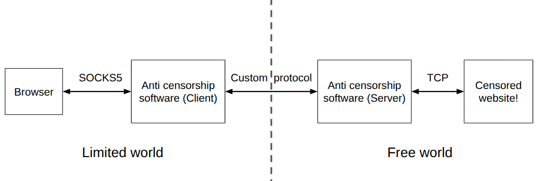
Now, there are infinite ways you can implement that "custom protocol" part. I'll list some of them here. I won't go into the details since you probably already have good clues about how each of them can be implemented. The general idea is what you need to know:
-
The custom proxy might be a simple protocol hidden inside an HTTPS request on port 443, which from our side looks just like an ordinary web request. Since the body of HTTPS requests is encrypted, an outsider may not be able to distinguish your traffic from other HTTPS requests. There are dozens of different ways and implementations of such a protocol that you can study.
-
Imagine the bad guy has completely shut down the internet and only allows you to use some kind of internal network (intranet). He provides his own "eavesdropped" messenger, which luckily can still be used to communicate with people outside the country. You can exploit that messenger to pass traffic to a server that is listening to the messenger on a free network. Just convert the bytes the browser sends through SOCKS5 into a base64 encoding or something similar (which the messenger allows you to transfer), read the messages on the second server, and respond accordingly. This is something people actually implemented during Iran's protests in 2022. See how creative people can get under severe limitations!
-
Now imagine the intranet no longer exists either. There is still hope. If you are still able to communicate with people outside the restricted area in any way, you may still automate packet transfer and implement your own custom protocol. For example, imagine phone calls are still available. As mentioned in Chapter 2, you can transmit data using sound waves. What if you write software that encodes the packets you receive through the SOCKS5 proxy from your browser into sound, and transmit that sound through your phone line to a server listening on the other side? That server could decode what it hears and send responses back. You could literally transfer a video through your favorite messenger without feeling that you are connected through such an unusual medium.
-
Here is another clever way people managed to connect to the internet during Iran's 2026 protests without transferring packets through a strange medium: the DNS protocol. DNS is probably the costliest service to block and likely the last thing the bad guy can disable. I do not yet know the exact reason, but somehow the bad guy cannot easily block DNS requests (even those going outside). For example, if you try to resolve the address
hello-my-dear-proxy-protocol.my-domain.com, even through the bad guy's internet provider DNS server, it will still ask the nameserver ofmy-domain.comfor the IP address ofhello-my-dear-proxy-protocol.my-domain.com, even if you have zero access tomy-domain.com. See? You were able to send something (the stringhello-my-dear-proxy-protocol) to a server you otherwise cannot access. Now imagine placing your browser packets inside those subdomains and having your DNS server respond with response packets. Pretty cool, right? This method is known as DNS Tunnel Tool (DNSTT) in case you want to learn more.
A true cypherpunk will always find a way to stay connected. I hope these ideas help ensure your voice never gets cut off!
Fly!
Music of the chapter: Space Oddity - By David Bowie
The Software-Engineer's world of unknowns!
Throughout my career in software-engineering, I have always had avoided engineering-activities which involved any interactions with the Physical world (Except a short period of time when I was working on line-following robots as a high-school student). That's partly because I live in an economically poor country, where modern industries are nearly non-existent and you can't find a lot of companies building cyber-physical systems (Systems composed of a software, controlling/sensing a physical thing), except when politics is involved, if you know what I mean.
Unlike pure software engineering, where you can never run out of characters, building software that interacts with the real-world, involves physical objects, things that you can touch and feel, and the unfortunate truth about non-imaginary objects is that, they cost money, and they can break, which means, you can't experiment as much as a software with them (Unless you are a rich engineer, having a giant laboratory inside your house, with plenty of money)
I have never been that rich, and I also couldn't find any company doing respectful cyberphysical projects in my country either. Therefore I have never had the opportunity to unleash my passion for classical fields of engineering, in which you have to actually build something that can be touched. You can see throughout this book that I'm a great fan of computer simulations though! This chapter is all about the mechanical/electrical world sorrounding us, and how computation can help us understand and control it better!
New is always better
I named this chapter of the book as "Fly", because flying is probably one of the most amazing and spiritual dreams of humans that has come to reality, and computers are one of the most important components of the flying-machines we have today. Humans could never land on moon without computers.
I would like to start this chapter by mentioning two of the most ambitious companies, created by the American multi-billionaire entrepreneur, Elon Musk (Good to know, he was initially a computer programmer!), at the time this book is written. Tesla and SpaceX, are companies that are producing cyberphysical products, one is building self-driving cars and the other is building rockets, aiming to make humans multi-planetary species.
When Elon Musk started those companies, it wasn't obvious at all that they'll become successful. Who could think that a private rocket-building company could beat the government funded NASA that once put humans on the moon? That's also true for Tesla, there were plenty of automobile companies with decades of experience, even in designing electric cars, but how did Tesla beat them all? Besides the reason that Elon himself is one of the most ambitious people of our time, which is enough for making a risky business successful, there is a more important reason why those two companies become insanely successful: It's much easier to experiment new stuff when your business is still small!
It's too risky for an already giant business to switch and explore new ways of building things. When companies grow, they start to become heavily beurocratical, which slows things down by a lot. That also makes sense, because, as your business grows, taking giant risks will also become more dangerous. That's why startups are so fast, they are small, and there is plenty of room for making mistakes. SpaceX didn't have all those boring stuff, it only had a few bright-minded people, exploring new ways of building rockets, without being scared too much of the failures.
My point is, old technology isn't always taking the best approach in doing stuff, in fact, old technology is pretty bad, because when engineers were designing the old technology, they didn't have the knowledge and experience they have right now. So it makes sense a lot to get brave and try to redesign things that were working correctly and stabely even for a long time! (This is also true for our today's software standards, just imagine how would we design our OS and networking infrastructures if we could throw away something as sacred as UNIX or TCP/IP!)
Life in a Newtonian world
Building and experimenting cyber-physical systems is going to cost you a lot, and it makes sense to check if everything is going to work as expected, before building your prototype. Since your brand-new cars/airplanes/rockets/etc are going to live in our world, they are going to obey the laws of Physics of our world. So if you are willing to simulate them before doing serious experiments, you will have to apply the laws of physics on them, in a simulated environment.
Physics before apple hit the the Newton's head
Students nag that they would have much less to study if that damn apple never hit Newton's head, but the truth is, the science of Physics existed even before Newton formulate it in his precious works. Even if Newton never figured gravity, sooner or later, someone else would do it! So, what were the statements of "Physicists" before Newton, when you asked them to explain the mechanical phenomena we experience everyday?
Aristotle, the Greek scientist and philosopher who were living in 4th century B.C., was of the first famous scientists trying to explain the laws of motion. Surprisingly, Aristotle's laws of motion was left untouched and continued to rule physics for more than 2000 years. Galileo Galilei, the Italian polymath, was of the first people who was brave enough to make new statements about motion and to break the Aristotle's empire that ruled for so long.
Aristotle's law of motion states that:
- External forces are needed to keep an object moving
Although this statement seems funny and so wrong nowadays (It's the friction that stops objects moving), it was convincing people and scientists for more than two centuries! Put yourself in the shoes of people back then, how would you formulate physics, if you had never heard the laws of physics written by Newton?
Another remark of Aristotle's law of motion is that, heavier objects fall faster than light objects. Nowadays we know that's not the case too, and the reason a feather falls slower than a book is merely because of air friction.
Although Aristotle's opinion seem right, they are not right. Aristotle's biggest mistake is that, he wasn't aware of friction forces and he was ignoring air resistance. This is known as the Aristotle's Fallacy.
Galielo Galilei's law of inertia states that:
- If you put an object in the state of motion, it will move forever if no external forces are applied on it
And lastly we will reach to Newton's formulation of motion and gravity, which although is proven to be incorrect by legends like Albert Einstein, is still accurate enough to explain and predict most of the macroscopic motions happening in our universe. The physics of motions discovered by Newton is still a fundamental guide for us to build cars, airplanes and rockets that can bring humans on the moon and put satellites in the space.
Newton was a legend. Not only he discovered a very accurate theory for motion, he also invented (Co-invented?) a fresh mathematical tool that has made significant contributions to the other fields of science too. This field of mathermatics is known as Calculus. We explained the basica of differentiation and integration in the previous chapters, so let's jump to the Newton's laws:
[TODO]
Perhaps the most important discovery of Newton is his famous formula \(F=ma\) which explains how the force applied to an object, the mass and its acceleration are related to each other.
\(v=\frac{dx}{dt}\)
\(a=\frac{dv}{dt}\)
\(x=\int{\int{a.dt}}=\frac{1}{2}at^2+v_0t+x_0\)
I recall once I was watching a science-fiction movie, in which an astronaut lost his rope handle and started to slowly get attracted by a planet nearby. His friends tried to save him but he was already too far from them, practically impossible for them to save him. His nuzzles (They are connected to an astronaut dress, allowing them to move in the space, where friction is not present) were also out of fuel, so he couldn't fight gravitation in any way, and he knew it. He knew his destiny and the fact that he is soon going to fall into the planet with a freaking high speed and die with pain.
He said goodbye to his friends, and commited suicide by removing his helmet.
Perhaps the most exciting outcome of Newton's formulation of gravity, is its explanation of why moon doesn't fall on the earth. This question was always a mystery, but Newton's discovery made it look very obvious!
Just like how we learnt everything in this book, a good way to understand the concept could be yet another computer simulation!
Here we are going to build a program, which can simulate a system of planets, purely by applying Newton's gravity forces on each of them. We will see if we can have an "orbiting" behavior by just letting planets to attract each other.
Throughout our series of simulations in this chapter, we'll use the vector classes we defined in the 3rd chapter. Our simulations will be done in a 2D world, since it will be enough for understanding the concept. Adding the 3rd dimension could be an optional feature which you can implement later!
Let's get to the keyboard! Surprisingly, there are only two formula you'll need to use in order to predict the movement of masses in the space:
- Law of gravity: how strong objects attract each other, given their masses and distance between them?
- \(\vec{F}=m\vec{a}\): the acceleration an object gets when a force is applied.
We first need a model of an object in space. Let's call it a Planet (A moon is not technically not a planet, but let's call all space objects in our simulation as Planets for simplicity).
A planet has a position in our 2D spcae. It also has a mass. Given the law of intertia, we can claim that, the velocity of the planet, is indeed an important property of the planet which doesn't change over time (Unless forces are applied to it) so, our model of a planet can be described as a Python class:
class Planet:
    def __init__(self, position, velocity, mass):
        self.position = poistion
        self.velocity = velocity
        self.mass = mass
Assuming there are no gravitational forces yet, they would continue moving on a straight line according to their velocity. Let's update the position of the planets in a loop in intervals of dt seconds:
planets = [Planet(...)]
dt = 0.001
t = 0
for p in planets:
    p.position += p.velocity * dt
    t += dt
You can also 2D render the planets as filled circles on your screen. They'll be moving on straight lines as expected!
Now let's apply gravity forces and make this more interesting. An important thing you should be aware of is that when you put 2 (Or more) planets near each other, they will both start attracting each other at the same time. You can't calculate the forces applied on \(p_1\), update its position, and then go for \(p_2\), because when you change \(p_1\)'s position, the force applied on \(p_2\) will be different, compared to when the position was not updated. In fact, the state-change of \(p_2\) is only dependent on the old/original state of \(p_1\), not the new calculated one. If you don't consider this, your simulatation will get slightly inaccurate. What you have to do is to first calculate all the forces applied to each planet (Without changing their positions), and then apply the side-effects (Positional changes) instantiously:
[TODO]
Remember I mentioned we are aiming to land a man on the moon? I wasn't kidding. Our solar system simulator could be a nice environment for experimenting a rocket launch that want to reach and land on the moon.
There will be many challenges:
- Our fuel will be limited.
- Escaping the source-planet's gravity is not easy.
- We can't expect the target planet to be in its initial position after launching.
- The rocket is launched with an initial velocity due to the source planets rotation.
- etc
Exciting Electronics
I started to admire the joy of programming computer in very young ages, but even before that, I was a fan of toy electorical kits. I used to buy ans solder them back then. I always wanted to know how the circuit of a blinking LED works for example. Why? Because understanding them was the first step to my dream of designing the circuits of my own. Unfortunately, I couldn't find appropriate resources that could convince a kid why a circuit like that works, and how he can get creative and build circuits of his own, by putting the right components in the right places.
So, electronics, and the way it works, remained a secret to me for years, and one of the reasons I gave up and switched my focus on building software was that, computer programming is much easier. Even after 15 years, and multiple tries in reading different books on electronics, I'm still afraid to say that I'm still not capable of designing a circuit as simple as a blinker all by myself, without cheating from other circuits, and that's one of the reasons I decided to write this chapter; to finally break the curse and learn this complciated, yet fascinating field of science.
How did I do it? Well I tried reading books in this topic, but I didn't find many of them useful. All books written in this matter (Even the good ones!) were starting explaining the laws of electricity and then describing different electronical components and their usecases in separate chapters. I'm not really a fan of learning things this way.
Here, I'm going to explain electronic circuit design with a bottom-up approach (Just like the way we discussed other fields of computer science). We will start by learning the history of electricity and how was the first experience of humans of electricity, and then describing the ways we can generate electricty, and then we will try to build useful stuff out of electricity. (From things as simple as light bulbs to comptuer!)
Along the way, we will also learn about different electronic components!
I would say that studying electricity is one of the most important foundations of human modernity, and just like the history of mechanical physics, electricity also has its own fascinating stories.
[TODO]
Here is one of the reasons I don't like some of the electronics tutorials out there: they will tell you exactly, what a resistor is, how it works and why it works, but they'll never tell you when and where you should put a resistor in your circuit, and how you should calculate the resistance needed, in practical examples! E.g. by only knowing the Ohm's law \(V=RI\), calculate the resistance needed to connect a 2V LED to a 5V battery!
Here is the golden fact many resources do not directly tell you (Or do not emphasize as much as I'm going to do!), you can assume that any electronical component (Including LEDs) that consume electricity are acting like resistors (Even a piece of wire is a resistor). If they weren't resistors, they could consume infinite electrical current, even with very low voltages.
How to push the electrons?
Before jumping straight to the things you can do with electricity, it's good to know how electricity is generated. There are various ways you can get a steady stream of electrons in your circuit. Batteries for example, they give you a potential difference on their poles using chemical reactions, and unfortunately, they will run out of energy after sometime. Unlike batteries, the source of electricity we get in our homes isn't generated by chemical reactions, but is the result of spinning a magnet inside a coil of wire. You can try it yourself at home! Humans have discovered somehow that, if you move/spin a magnet inside a wire coil, you will push the electrons in the wire and will have electrical current, which is able to turn a light-source on!
Now, you don't need to spin that magnet by hand, you can let the nature do it for you. You can connect a propeller to the magnet, causing it to spin when wind is blown. That's in fact how wind turbines convert wind into electricity!
Even if you don't have wind, you can use artificially-generated wind (By burning fuel or even doing nuclear reaction, to make water hot and vapourize it, leading to a high-pressure steam of water vapour) to spin the coil for you.
Unfortunately, the voltage/current generated using this technique alternates like a sine function, and although we can still directly use such a current for heating things (E.g light-bulbs), it can't be used for driving anything digital. Such a power supply is known as an AC supply (AC stants for, alternating current!)
If you plot the output voltage of the two ends of a AC power source, you will get something like this (Negative voltage means that the poles are reversed and the current will flow in the reversed direction):
[TODO]
The best thing we can do right now is to try to limit the voltage/current to only one direction (Our digital circuits may handle frequent drops and increases in the input voltage, but they may not tolerate when the voltage/current is completely reversed).
There is an electronic component, named Diode, which allows the flow of electrons in a single direction. Let's not bother ourselves on how/why it works, but instead, focus on its application and see if we can use it for something practical, such as converting an AC voltage to a DC one.
By connecting a diode to a AC source, we will get an output like this:
[TODO]
Although it's a good step towards our goal, you can see that half of the energy is being unused. Now let's reverse the direction of the diode and see what happens:
[TODO]
Is there any way we can add these two signals to get an output like this?
[TODO]
Before reading the answer, try to design such a circuit yourself! (Hint: you will need 4 diodes) You will probably reach to a circuit like this:
These specific combination of diodes is called a "bridge", and although it looks different from what we drew, it actually is the same!
So far, we have been able to allow an AC voltage to flow on only a single direction, but the output voltage we are getting is not yet stable. It alternates between 0 and the voltage of the AC supply. Is there any way we can convert an unstable/alternating DC to a stable one? If you look closed to the output voltage, you will see that there are "gaps" in the voltage that need to be filled. It would be good of there was an electronic component that could temporarily store the unused voltage of an alternating DC and release an smoother voltage when the energy is actually being consumed. Fortunately, there is such a component! It is called a "capacitor" and is able to store the energy for you like a battery.
The output voltage is not much better and smoother than the version without a capacitor. Though it's still not completely flat, as you can still see some gaps in the voltage, but it still is much better than the previous version!
In case you use capacitors with higher capacitance (The unit used for capactitors is Farad), the capacitor will be able to store more energy in it, and keep the voltage up for you for a longer time, leading to smaller gaps.
You just saw that capacitors have obvious use cases, here we used them as a temporary storage of energy, in order to fill the voltage gaps in the process of converting an AC voltage to a DC one, but they have other usecases too! Before examining them, let's get a deeper undestanding on what a capacitor is and how it is made!
Capacitors are simple two conductor plates that are very close to each other (You can see that from the symbol of a capacitor too!). They are very close, but not connected! If you connect a voltage source to a capacitor, you might think that no current will flow (As the plates are not connected to each other), but surprisingly, current will flow! The voltage source will slowly grab electrons from one side and put it on the other side of the plate, effectively making a potential difference between the plates. The process will eventually make the potential difference between the plates equal with the potential difference of the voltage source, and after that, the battery and capacitor will cancel each other and current will stop flowing! The capacitor is charged!
If you plot the current flowing in a circuit containing a battery to a capacitor, you will see that in the very first moment, the capacitor will act like a wire, it allows the current as if there is no capacitor, and as time passes, the potential difference between the plates will slowly increase, slowly cancelling out the potential difference of the battery, leading to less and less current flowing, and finally, the current will completely stop flowing!
There is one very important fact when analyzing capacitors: analyzing them is not possible if you do not assume there is a resistor in the way! Even wires have some amount of resistance, so you may never find a capacitor connected to a battery wihtout a resistor in between! In fact, such a circuit is meaningless, as it does not exist:
Now what happens if the resistance of the resistor along the way increases? The capacitor will get charged/discharged with higher delay! You can either increase the resistor in the way, or the capacity of the capacitor itself, in order to make this charging/discharging delay higher. So the amount of time needed for a pair of resistor and capacitor getting charged is directly proportional to both the resistance and capacitance of the components, and that's why we refer pairs of resistors and capacitors as RC circuits!
We saw that capacitors can also help you to have some kind of "delayed" voltage source, which can sometimes become handy. As an example, imagine you want to turn an LED on, with a delay. If you connect the LED directly to the pins of the capacitor, the LED will slowly become bright and brighter, until the capacitor is fully charged. Here, although the LED got its maximum brightness with a delay, it isn't exactly what we wanted. We want the LED to stay off for some time, and then suddenly become lit!.
Revisting transistors
Remember transistors we discussed in the first chapter? Transistors might come handy here! A transistor is a electrically controlled switch. It has a "base" pin, that when become enough voltage to pass a threshold, will suddenly allow current to flow between in emitter an collector wire. Now let's connect the delayed voltage-source we made out of a resistor-capacitor, to the base pin of a transistor. The delayed voltage will eventually reach the transistor's threshold and then will suddenly turn the LED on!
Breaking the curse
Ok, we just saw four of the most useful electronical components so far, and we also saw some of the very obvious usecases of these components. Now it's a good time to explore the "Hello World!" circuit of the world of electronics! A Astable Vibrator!
While the name of this circuit seems scary, the circuit itself doesn't do anything extraordinary. It's basically a 2 LED blinker! Unfortunately, although the circuit does such a simple thing, it's surprisingly complicated for those just started to learn electronics! You have to have a very accurate understanding of resistors, capacitors and transistors in order to understand how a Astable Vibrator. Fortunately, since we now understand how we can turn an LED on with a delay, it's not super hard to understand this new circuit.
Our approach in studying a blinker circuit is very similar with how we learned other things in this book. Instead of looking at a astable vibrator's circuit and trying to understand it, we will go through a bottom-up approach, and will try to build a blinker circuit from scratch, using our current knowledge!
Ohm and Kirchhoff's Laws
When analyzing circuits, there are two important laws in electricity that can help you to calculate the potential difference between any two points, or the amount of current flowing in any point, and these master laws are:
- The Ohm's law
- The Kirchhoff's law
The Ohm's law, as previously discussed, describes the relation between the voltage, resistance and current.
\(V=RI\)
The Kirchhoff's law on the other hand, states that the sum of incoming and outgoing current to/from a point in a circuit is always equal. Assuming that we state an outgoing current as an incoming current that is negative, we can define Kirchhoff's current law: the algebraic sum of currents that meet at a point is zero.
Now let's see how these laws can help us analyze a circuit.
Analyzing circuits
Analyzing an electronic circuit is all about predicting and calculating the amount of current and voltage of every point in the circuiy. Obviously, the voltage of every two points directly connected through a wire is always equal. Electronic components are connected together through wires, and your circuit consists of junctions where 2 or more components meet. Since the voltage value of all the points in a junction are equal, there is only one voltage to be calculated. Let's refer to this intersection points of components as nodes. In the example circuit in figure X, there are X nodes. Our goal is to calculate the voltage of all the nodes in any given time.
An electronic component can be defined by the amount of current it allows to pass given the voltages applied on its pins. For example, a resistor's ability to pass electrons is linearly dependent to the amount of voltage difference applied on its pins.
\(i=\frac{V_a - V_b}{R}\)
There are components that have non-linear behaviors too! For example, a diode has a exponential behavior. The more voltage difference applied in correct direction, it allows exponentially more current to pass, and apply the voltage difference in reverse direction, and it will become like a resistor with infinite resistance.
\(i=ae^{b(V_a - V_b)}\)
(The coefficients \(a\) and \(b\) depends on the diode)
There are also some electronic components with time-dependent behaviors. Their current output depends on the input applied to them in the past too. A capactitor for example. If the capacitor is already charged, it allows no current, while an uncharged capacitor allows infinite current. We can also define a capacitor's behavior through a formula:
\(i=C\frac{d(V_a-V_b)}{dt}\)
I would like to introduce you a new, imaginary source of electricity, referred as a current source. As opposed to voltage sources which try to keep the potential difference between two points on a specific number, current sources try to keep the current stable on a chosen number. Current sources are imaginary and do not exist in the real world. You can somehow emulate them though! Imagine building a "smart" voltage source that can measure the current and increase/decrease its voltage accordingly to keep the current on a specific number. As opposed to a voltage source where short circuits are not permitted, in current sources, you have to make sure that electrons coming out of the source will eventualy get back to the source. Otherwise, the zeroness of current will cause the ovltage to become infinity which definitely is not what we want!
The reason I'm introducing current sources is that, it's much easier to analyze circuits that use current-sources instead of voltage sources (For now!).
\(i = I\)
By summing all of currents flowing into each node, we will get a set of equations. Given Kirchhoff's law, we know that these functions must be equal to zero. This puts a constraint on the voltages of the nodes in out system, helping us to find the correct voltage of each node.
In other words, the problem of solving the circuit is reduced to finding the solution of a system of equations.
Newton, Newton everywhere!
Finding the roots of arbitrary functions has always been an interesting problem for ancient mathematicians. It's interesting to know that it took almost X years to find a general method for calculating the roots of a simple quadratic equation, let alone more complicated function!
Newton, besides doing Physics, has always been a pioneer in mathematics and one of his discoveries, was a numerical method for finding the roots of any arbitrary function (With known derivative). The method, which is known as Newton-Raphson nowadays (Thanks to the simplification Raphson did to the algorithm), is an iterative algorithm which tries to guess the root of the function, and make its guess better and better through iterations, until reaching to a final answer! Yes, Newton was doing machine-learning in 1600s, what a legend!
\(x_{n+1} = x_n - \frac{f(x_n)}{f'(x_n)}\)
Here is a Python code that tries to find the root of simple single-input/single-output function through this method:
\(f(x) = x^3 - 4x^2 - x + 5\)
\(f'(x) = 3x^2 - 8x - 1\)
def f(x):
    return x**3 - 4 * x**2 - x + 5


def f_prime(x):
    return 3 * x**2 - 8 * x - 1


guess = 0.5

for _ in range(10):
    guess = guess - f(guess) / f_prime(guess)

print(guess, f(guess))
And the output is: 1.16296185677753 0.0
Fortunately, a very similar approach can be applied for finding the root of a multi-input/multi-output function. (Here, a electronic circuit can be mapped into a multi-input/multi-output function, where the inputs are voltages of the nodes, and the outputs are the sum of currents flowing into the nodes)
The derivative of a multi-input/multi-output function is known as the Jacobian of that function. We have been working with Jacobians while training neural-networks too!
Assuming that our function accepts \(3\) inputs and gives out \(3\) outputs, the Jacobian of that function will be a \(3 \times 3\) matrix:
\[F'(X) = \begin{bmatrix} \frac{\partial f_0(X)}{\partial x_0} & \frac{\partial f_0(X)}{\partial x_1} & \frac{\partial f_0(X)}{\partial x_2} \\ \frac{\partial f_1(X)}{\partial x_0} & \frac{\partial f_1(X)}{\partial x_1} & \frac{\partial f_1(X)}{\partial x_2} \\ \frac{\partial f_2(X)}{\partial x_0} & \frac{\partial f_2(X)}{\partial x_1} & \frac{\partial f_2(X)}{\partial x_2} \end{bmatrix}\]
Where: \(X = (x_0, x_1, x_2)\) and \(F(X) = (f_0(X), f_1(X), f_2(X))\)
In the Newton Raphson method, in each iteration, we were dividing the result of the function at previous guess, by the result of the derivative of the function at that guess. Since the derivative of our function is now a matrix, we have to find the inverse of the Jacobian matrix in order to perform the formula. The iteration formula becomes:
\[X_{n+1} = X_n - F'(X_n)^{-1}.F(X_n)\]
Now, the only remaining challenge is coverting a circuit to a multi-input/multi-output function, and then, by finding the root of that function through the Newton-Raphson method, the circuit is solved!
Let's dive into the implementation:
[TODO]
Let's assume we have \(n\) nodes. Applying the Kirchhoff's law will give us \(n\) equations that need to be zeroed (See the number of inputs and outputs in our multi-input/multi-output function is equal).
Each function is in fact the sum of contribution of different components connected to it. So a first step could be creating a framework in which components may add their contributions to the node functions.
Let's assume each function is represented as a sum of sub-functions (If there are \(k\) components connected to the \(i\)th node, the corresponding node function will be the sum of \(k\) sub-functions: \(f_i(X) = f_{i,0}(X) + f_{i,1}(X) + \dots + f_{i,k-1}(X)\))
Since the nodes are simple variables that need to be calculated by a solver, it might make more sense to instantiate Var instances when introducing new nodes.
class Var:
    def __init__(self, index):
        self.index = index  # Keep track of the index of variable
        self.old_value = 0
        self.value = 0
Circuits
class Circuit:
    def __init__(self):
        self.gnd = Var(None)
        self.vars = []
        self.components = []

    def new_var(self) -> Var:
        n = Var(len(self.vars))
        self.vars.append(n)
        return n

    def new_component(self, comp: Component):
        self.components.append(comp)

    def solver(self, dt) -> Solver:
        solver = Solver(self.vars, dt)
        for comp in self.components:
            comp.apply(solver)
        return solver
Solver
class ConvergenceError(Exception):
    pass


class Solver:
    def __init__(self, variables, dt) -> None:
        self.variables = variables
        self.funcs = [list() for _ in range(len(variables))]
        self.derivs = [dict() for _ in range(len(variables))]
        self.dt = dt
        self.t = 0
        self.randomness = random.random() - 0.5

    def add_func(self, ind, f):
        if ind is not None:
            self.funcs[ind].append(f)

    def add_deriv(self, ind, by_ind, f):
        if ind is not None:
            if by_ind not in self.derivs[ind]:
                self.derivs[ind][by_ind] = []
            self.derivs[ind][by_ind].append(f)

    def jacobian(self):
        res = []
        for f in range(len(self.funcs)):
            row = []
            for v in range(len(self.funcs)):
                row.append(self.eval_deriv(f, v))
            res.append(row)
        return res

    def eval(self, ind):
        res = 0
        for f in self.funcs[ind]:
            res += f()
        return res

    def eval_deriv(self, ind, by_ind):
        res = 0
        if by_ind in self.derivs[ind]:
            for f in self.derivs[ind][by_ind]:
                res += f()
        return res

    def is_solved(self):
        for i in range(len(self.funcs)):
            if not numpy.allclose(self.eval(i), 0):
                return False
        return True

    def step(self, max_iters=1000, max_tries=100, alpha=1):
        solved = False
        for _ in range(max_tries):
            try:
                iters = 0
                while not solved:
                    x = [v.value for v in self.variables]
                    f_x = [self.eval(v.index) for v in self.variables]
                    f_prime_x = self.jacobian()
                    f_prime_x_inv = numpy.linalg.inv(f_prime_x)
                    x = x - alpha * numpy.dot(f_prime_x_inv, f_x)
                    for v in self.variables:
                        v.value = x[v.index]
                    solved = self.is_solved()
                    if iters >= max_iters:
                        raise ConvergenceError
                    iters += 1
            except (OverflowError, ConvergenceError, numpy.linalg.LinAlgError):
                # Start from another random solution
                for v in self.variables:
                    v.value = random.random()
            if solved:
                for v in self.variables:
                    v.old_value = v.value
                self.t += self.dt
                self.randomness = random.random() - 0.5
                return
        raise ConvergenceError
Components are equations
class Component:
    def __init__(self):
        pass

    def apply(self, solver: Solver):
        raise NotImplemented
Current Source
A current-source equation makes sure that the amount of current flowing through its pins is equal with some value, through two equations:
- \(I_a - i = 0\)
- \(i - I_b = 0\)
class CurrentSource(Component):
    def __init__(self, amps, a: Var, b: Var):
        super().__init__()
        self.amps = amps
        self.a = a
        self.b = b

    def apply(self, solver: Solver):
        solver.add_func(self.a.index, lambda: self.amps)
        solver.add_func(self.b.index, lambda: -self.amps)
Voltage Source
A voltage-source equation makes sure the potential difference between two points \(V_a\) and \(V_b\) is always equal with \(v\), by adding 3 equations to your system. (A temporary variable \(i\) is also introduced, representing the amount of current being flown through the component):
- \(I_a - i = 0\)
- \(i - I_b = 0\)
- \(V_a - V_b - v = 0\)
Note that, since we are using the Kirchhoff's law to solve the circuits, all components need to define the amount of current going in and out the circuit, and how does it relate \(I_a\) and \(I_b\) with each other. In a voltage-source (Like any other 2-pin component), the amount if input current is equal with the amount of output current. Naming that auxillary variable to \(i\), the relation between \(I_a\) and \(I_b\) is defined using the first and second equation. In fact, the variable \(i\) has no direct usage but to relate \(I_a\) and \(I_b\) with each other!
class VoltageSource(Component):
    def __init__(self, volts, a: Var, b: Var, i: Var):
        super().__init__()
        self.volts = volts
        self.a = a
        self.b = b
        self.i = i

    def apply(self, solver: Solver):
        solver.add_func(self.a.index, lambda: self.i.value)
        solver.add_func(self.b.index, lambda: -self.i.value)
        solver.add_func(
            self.i.index,
            lambda: self.b.value
            - self.a.value
            - self.volts,
        )

        solver.add_deriv(self.a.index, self.i.index, lambda: 1)
        solver.add_deriv(self.b.index, self.i.index, lambda: -1)
        solver.add_deriv(self.i.index, self.a.index, lambda: -1)
        solver.add_deriv(self.i.index, self.b.index, lambda: 1)
Resistor
The resistor component makes sure that the amount of current being flown through it is linearly dependent on the voltage-difference applied to it. In other words: \(i = \frac{V_a - V_b}{R}\). It does so by applying two equations:
- \(I_a - \frac{V_a - V_b}{R} = 0\)
- \(\frac{V_a - V_b}{R} - I_b = 0\)
class Resistor(Component):
    def __init__(self, ohms, a: Var, b: Var):
        super().__init__()
        self.ohms = ohms
        self.a = a
        self.b = b

    def apply(self, solver: Solver):
        solver.add_func(self.a.index, lambda: (self.a.value - self.b.value) / self.ohms)
        solver.add_func(self.b.index, lambda: (self.b.value - self.a.value) / self.ohms)

        solver.add_deriv(self.a.index, self.a.index, lambda: 1 / self.ohms)
        solver.add_deriv(self.a.index, self.b.index, lambda: -1 / self.ohms)
        solver.add_deriv(self.b.index, self.a.index, lambda: -1 / self.ohms)
        solver.add_deriv(self.b.index, self.b.index, lambda: 1 / self.ohms)
Capacitor
Unlike the components discussed so-far, a capacitor is a component that has memory (Its current behavior is dependent on voltages previously applied to it). A charged capacitor has a different behavior compared to a discharged one. A charged capacitor will resist against current and a discharged one acts like a wire. We somehow need to bring this memory-behavior on the table. We do this by introducing a old_value field for our variables, and use them as equations. Note that the old values of variables act as constant numbers (When taking derivatives). I.e: \(\frac{d(V-V_{old}}{dt} = \frac{dV}{dt}\)
A capacitor can be modeled using 2 equations:
- \(I_a - \frac{(V_a + V_b)-(V_{a_{old}} + V_{b_{old}})}{dt} \times C = 0\)
- \(\frac{(V_a + V_b)-(V_{a_{old}} + V_{b_{old}})}{dt} \times C - I_b = 0\)
class Capacitor(Component):
    def __init__(self, farads, a: Var, b: Var):
        super().__init__()
        self.farads = farads
        self.a = a
        self.b = b

    def apply(self, solver: Solver):
        solver.add_func(
            self.a.index,
            lambda: (
                (self.a.value - self.b.value) - (self.a.old_value - self.b.old_value)
            )
            / solver.dt
            * self.farads,
        )
        solver.add_func(
            self.b.index,
            lambda: -(
                (self.a.value - self.b.value) - (self.a.old_value - self.b.old_value)
            )
            / solver.dt
            * self.farads,
        )

        solver.add_deriv(self.a.index, self.a.index, lambda: self.farads / solver.dt)
        solver.add_deriv(self.a.index, self.b.index, lambda: -self.farads / solver.dt)
        solver.add_deriv(self.b.index, self.a.index, lambda: -self.farads / solver.dt)
        solver.add_deriv(self.b.index, self.b.index, lambda: self.farads / solver.dt)
Inductor
class Inductor(Component):
    def __init__(self, henries, a: Var, b: Var, i: Var):
        super().__init__()
        self.henries = henries
        self.a = a
        self.b = b
        self.i = i

    def apply(self, solver: Solver):
        solver.add_func(self.a.index, lambda: self.i.value)
        solver.add_func(self.b.index, lambda: -self.i.value)
        solver.add_func(
            self.i.index,
            lambda: (self.i.value - self.i.old_value) / solver.dt * self.henries
            - (self.a.value - self.b.value),
        )

        solver.add_deriv(self.a.index, self.i.index, lambda: 1)
        solver.add_deriv(self.b.index, self.i.index, lambda: -1)
        solver.add_deriv(self.i.index, self.i.index, lambda: self.henries / solver.dt)
        solver.add_deriv(self.i.index, self.a.index, lambda: -1)
        solver.add_deriv(self.i.index, self.b.index, lambda: 1)
Diode
Diode is a one-way current blocker. Apply the voltage on right direction and the current will go up to infinity (I.e zero resistance), and apply it in the reverse direction and the current becomes zero (I.e infinite resistance). Such a behavior can be perfectly modeled with a exponentation function.
class Diode(Component):
    def __init__(self, coeff_in, coeff_out, a: Var, b: Var):
        super().__init__()
        self.coeff_in = coeff_in
        self.coeff_out = coeff_out
        self.a = a
        self.b = b

    def apply(self, solver: Solver):
        solver.add_func(
            self.a.index,
            lambda: (math.exp((self.a.value - self.b.value) * self.coeff_in) - 1)
            * self.coeff_out,
        )
        solver.add_func(
            self.b.index,
            lambda: -(math.exp((self.a.value - self.b.value) * self.coeff_in) - 1)
            * self.coeff_out,
        )

        solver.add_deriv(
            self.a.index,
            self.a.index,
            lambda: math.exp((self.a.value - self.b.value) * self.coeff_in)
            * self.coeff_out
            * self.coeff_in,
        )
        solver.add_deriv(
            self.a.index,
            self.b.index,
            lambda: -math.exp((self.a.value - self.b.value) * self.coeff_in)
            * self.coeff_out
            * self.coeff_in,
        )
        solver.add_deriv(
            self.b.index,
            self.a.index,
            lambda: -math.exp((self.a.value - self.b.value) * self.coeff_in)
            * self.coeff_out
            * self.coeff_in,
        )
        solver.add_deriv(
            self.b.index,
            self.b.index,
            lambda: math.exp((self.a.value - self.b.value) * self.coeff_in)
            * self.coeff_out
            * self.coeff_in,
        )
Transistor
class Bjt(Component):
    def __init__(
        self,
        coeff_in,
        coeff_out,
        beta_r,
        beta_f,
        base: Var,
        collector: Var,
        emitter: Var,
    ):
        super().__init__()
        self.coeff_in = coeff_in
        self.coeff_out = coeff_out
        self.base = base
        self.emitter = emitter
        self.collector = collector
        self.beta_r = beta_r
        self.beta_f = beta_f

    def apply(self, solver: Solver):
        solver.add_func(
            self.collector.index,
            lambda: (
                (
                    math.exp((self.base.value - self.emitter.value) * self.coeff_in)
                    - math.exp((self.base.value - self.collector.value) * self.coeff_in)
                )
                - (1 / self.beta_r)
                * (
                    math.exp((self.base.value - self.collector.value) * self.coeff_in)
                    - 1
                )
            )
            * self.coeff_out,
        )
        solver.add_func(
            self.base.index,
            lambda: (
                (1 / self.beta_f)
                * (math.exp((self.base.value - self.emitter.value) * self.coeff_in) - 1)
                + (1 / self.beta_r)
                * (
                    math.exp((self.base.value - self.collector.value) * self.coeff_in)
                    - 1
                )
            )
            * self.coeff_out,
        )
        solver.add_func(
            self.emitter.index,
            lambda: -(
                (
                    math.exp((self.base.value - self.emitter.value) * self.coeff_in)
                    - math.exp((self.base.value - self.collector.value) * self.coeff_in)
                )
                + (1 / self.beta_f)
                * (math.exp((self.base.value - self.emitter.value) * self.coeff_in) - 1)
            )
            * self.coeff_out,
        )

        solver.add_deriv(
            self.collector.index,
            self.collector.index,
            lambda: math.exp((self.base.value - self.collector.value) * self.coeff_in)
            * self.coeff_out
            * self.coeff_in
            + math.exp((self.base.value - self.collector.value) * self.coeff_in)
            * self.coeff_out
            * self.coeff_in
            * (1 / self.beta_r),
        )
        solver.add_deriv(
            self.collector.index,
            self.base.index,
            lambda: math.exp((self.base.value - self.emitter.value) * self.coeff_in)
            * self.coeff_out
            * self.coeff_in
            - math.exp((self.base.value - self.collector.value) * self.coeff_in)
            * self.coeff_out
            * self.coeff_in
            - math.exp((self.base.value - self.collector.value) * self.coeff_in)
            * self.coeff_out
            * self.coeff_in
            * (1 / self.beta_r),
        )
        solver.add_deriv(
            self.collector.index,
            self.emitter.index,
            lambda: -math.exp((self.base.value - self.emitter.value) * self.coeff_in)
            * self.coeff_out
            * self.coeff_in,
        )

        solver.add_deriv(
            self.base.index,
            self.collector.index,
            lambda: -(1 / self.beta_r)
            * math.exp((self.base.value - self.collector.value) * self.coeff_in)
            * self.coeff_out
            * self.coeff_in,
        )
        solver.add_deriv(
            self.base.index,
            self.base.index,
            lambda: (1 / self.beta_f)
            * math.exp((self.base.value - self.emitter.value) * self.coeff_in)
            * self.coeff_out
            * self.coeff_in
            + (1 / self.beta_r)
            * math.exp((self.base.value - self.collector.value) * self.coeff_in)
            * self.coeff_out
            * self.coeff_in,
        )
        solver.add_deriv(
            self.base.index,
            self.emitter.index,
            lambda: -(1 / self.beta_f)
            * math.exp((self.base.value - self.emitter.value) * self.coeff_in)
            * self.coeff_out
            * self.coeff_in,
        )

        solver.add_deriv(
            self.emitter.index,
            self.collector.index,
            lambda: -math.exp((self.base.value - self.collector.value) * self.coeff_in)
            * self.coeff_out
            * self.coeff_in,
        )
        solver.add_deriv(
            self.emitter.index,
            self.base.index,
            lambda: -math.exp((self.base.value - self.emitter.value) * self.coeff_in)
            * self.coeff_out
            * self.coeff_in
            + math.exp((self.base.value - self.collector.value) * self.coeff_in)
            * self.coeff_out
            * self.coeff_in
            - (1 / self.beta_f)
            * math.exp((self.base.value - self.emitter.value) * self.coeff_in)
            * self.coeff_out
            * self.coeff_in,
        )
        solver.add_deriv(
            self.emitter.index,
            self.emitter.index,
            lambda: math.exp((self.base.value - self.emitter.value) * self.coeff_in)
            * self.coeff_out
            * self.coeff_in
            + (1 / self.beta_f)
            * math.exp((self.base.value - self.emitter.value) * self.coeff_in)
            * self.coeff_out
            * self.coeff_in,
        )
When stables and unstables meet!
Revisiting capacitors, we know they are elements that resist against stability of the voltage applied to them. (E.g if you connect a DC voltage-source to them, they will slowly get charged and cancel out the voltage of the DC voltage source, resisting against flow of electrons)
On the other hand, inductors are components that resist against unstability of the current flowing in them. If you suddenly connect a voltage source to them, you may not see a sharp change in the current flowing in an inductor (As opposed to a capacitor, or even a simple resistor), but the current will go up slowly, and if you disconnect the voltage source, current will not get zero instantly, but it will slowly approach zero (Very similar to law of intertia in mechanics!)
In fact, both capacitors and inductors somehow store energy, but in different ways. A capacitor stores energy as a potential difference between its plates, but an inductor stores energy as a magnetic field inside a coil.
Both capacitors and inductors are kind of resistors. The capacitor's resistance is higher when the input voltage is stable (Infinite resistance on a DC voltage source and lower resistance in a AC voltage source or any form of alternationing voltages). On the other hand, an inductor's resistance is 0 when the voltage applied to it is stable, and it's resistance increases as it's input voltage source alternates faster (E.g a high-frequency AC voltage source)
In the circuit shown in figure X, if you apply DC voltages, the voltage of \(V_1\) in the circuit with capacitor will eventually become zero, while the voltage in the circuit with inductor will slowly increase and become \(V\). Now, replace the DC voltage source with a AC one and slowly increase its frequency, the situation will be reversed! You will see higher voltages in the capacitor circuit and lower voltages in the inductor circuit.
We can somehow claim that, capacitors are high-pass filters. They pass current better when their input alternates faster (I.e with higher frequency), whereas inductors are low-pass filters, since they allow better flow of electrons when the input signal is alternating slowly (Or no alternation at all).
Now, here is a fascinating idea: by combining a capacitor and an inductor together, we'll have a circuit that has minimum resistance in certain frequency! This magical frequency can be calculated using this formula:
\(f = \frac{1}{2 \pi \sqrt{LC}}\)
where \(C\) is the capacitor's capacitance in Farads and \(L\) is inductor's inductance in Henries.
Remember both capacitors and inductors could be used for storing energy? Not only you use a pair of capacitor and inductor for creating a dynamic resistor with minimized resistance in a certain frequency, but also you can trap energy in them, and that energy will oscillate between the capacitor and inductor with the same frequency! This means, you can build an alternating source of voltage with this magical pair, and that oscillation is something that has effects on the space around it. It makes disturbances that propagates in the space! (Recall the second chapter where we discussed waves)
The oscillation made by this loop can be routed to a long piece of metal, amplifying the impact it has in the space. A bigger surprise is that, if you have another capacitor-inductor loop (With same frequency) somewhere else, a slight oscillation will also be induced on the second loop. This revolutionary idea was first proposed by the German physicist, Heinrich Hertz.
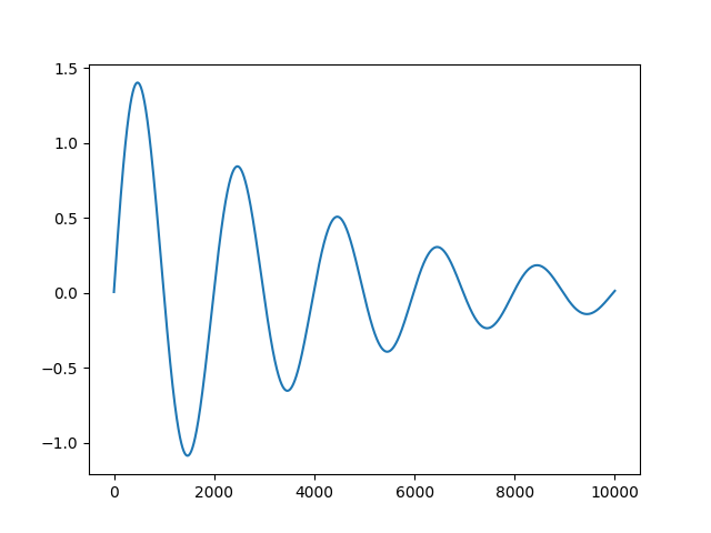 { width=300px }
Let's teleport
Now that we've been able to recognize presence of some frequency in the space through an antenna, a good next step might be to turn an LED one when the frequency is present. Unfortunately, as an electromagnetic wave propagates through the space (Assume the energy is on the surface of a sphere that is getting bigger linearly, the energy on the sphere is constant but the area is increasing, so the density of the energy per area will decrease, that's why a light-source will look less bright as you get farther from it), it loses its energy. So, the amplitude of the signal you receive on the other side is much smaller, so we have to somehow amplify it and retrieve the original, high-amplitude signal back, in order to make the signal large enough for turning an LED on.
What we are receiving in a RLC loop that is connected to an antenna, is a voltage resonance. This means that the loop will have a very small AC voltage when an electromagnetic wave (With the same frequency as the loop's resonant frequency) is present in the air. In order to turn an LED on, we need a DC voltage source. Remember how we were able to convert AC to DC in previous sections? Using the same ideas as before, we can limit the flow of current to a single direction with a diode, and fill the voltage gaps using a capacitor. This way, the presence of a wave is converted to a very small DC voltage source which can be detected, by a transistor! (Note: you might think that the capacitor will store the energy and keep it even when the signal is not present anymore, that is somehow true, but in practice, the output of the circuit is connected to some other element, consuming the energy stored in the capacitor, eventually zeroing the energy of the capacitor when the signal is not present anymore)
[IMG, rlc loop connected to a diode and capacitor]
The DC voltage source we receive from such a circuit is not enough at all for doing anything useful, but there is a powerful electronic component, transistor, which can detect a voltage as small as what you'll receive from a RLC loop, and let a much higher current flow from its collector to the emitter pin.
[IMG, RLC loop, with a transistor]
Transistors usually need a small, initial voltage on their base pin in order to get sensitive to voltage changes. (E.g the impact of increasing the voltage of the base pin from 1V to 1.1V is much higher than the impact of increasing it from 0V to 0.1V and that's because transistors allow exponentially more current to flow when their base voltage increase). So in order to make our circuit more sensitive to voltage changes, it might make sense to add some extra voltage to the base pin, using a pair of resistors (For voltage splitting).
[IMG: Biasing the transistor]
This simple can be used for sending binary data in distances, a morse-code for example!
Telephone revolution
Morse codes can be used for sending bit infomation. What if we want to send something like audio through space? Audio itself is a wave contatining many frequencies, and our circuit was able to recognize the presence of a wave with a certain frequency in the space.
Let's get back to our previous circuit. We were able to control the flow of electrons by a radio wave, but there is more to that circuit! By playing with our transmitter a bit, we will soon figure out that the more strong (Higher amplitude) the source signal is, the brighter the LED will get, which means, not only we can prevent/allow the flow of electrons, we can also control the amount of current flows per time! This means that the data we are sending through our transmitter doesn't necessarilly have to be single bits (On/offs), but they can also be floating-point values!
Waves themselves can be represented as streams of values, where each value shows the amplitude of the signal over time. Now, let's suppose the voice we are going to transfer is encoded as the strength of the retrieved signal. This kind of encoding is known as Amplitude Modulation or AM. This is exactly the same thing that happens in a AM radio receiver/transmitter, and our wave-recognizer circuit can actually receive AM signals already. If we connect the collector wire of the transistor to a speaker, you'll be able to hear the Amplitude Modulated sounds transmitted on that specific frequency. If we want to allow the user to listen to arbitrary frequencies, we'll need a RLC loop with variable resonant-frequency. The resonant-frequency can become variable if either the capacitor or the inductor becomes variable. A variable inductor is pretty straightforward: since an inductor is a wire coil, you can select how long of the coil you want to use in the circuit, as shown in the figure X.
[IMG: AM radio receiver]
[IMG: variable coil]
So far we have been able to detect signals and we didn't discussed much on how we can generate those signals. One easy way of generating such a signal is to charge a RLC loop with a voltage source and then disconnect it (You won't have alternations if you keep the voltage-source connected forever), so that the energy can swing in it. Unfortunately, the signal generated using this method is not a steady one and needs someone/something persistently connecting/disconnecting the voltage source to/from the RLC loop, otherwise the swing will not happen!
We have to think of a circuit which is able to oscillate for us forever, without needing someone to connect/disconnect the voltage-source, or at-least make the process automated. An example of such a circuit is the Astable Multivibrator circuit we discussed in the previous sections. An astable multivibrator generates a square-wave instead of a sine-wave, but that's ok! You can still detect the oscillations of an Astable Multivibrators in the space. In fact, if you take the FFT of a square-wave, you will see that the a sine wave of frequency \(f\) is presented in a square-wave of frequency \(f\), and the only problem is that, there are also other signals present. Those extra signals are harmonies of \(f\) (\(\dots,\frac{f}{8},\frac{f}{4},\frac{f}{2},2f,4f,8f,\dots\)).
Using square-waves as a medium for transmitting data, although works in practice, might cause you legal problems! That's because not all frequencies are allowed to be sent since they can interfere with the signals sent by other entities. A square wave is in fact composed of inifinitely many different sine-frequencies, an many of those are restricted by the governments! The police might might come and arrest you when sending square-waves powerful enough to interfere with the national radio/television for example!
There are more complicated circuits for generating sine-waves too, but for sake of simplicity, let's ignore the government for now (Hopefully this doesn't make governments angry) and use Astable Multivibrators as wave-generators.
We can model an antenna component in our simulator. Our antenna can be modeled as a component with an input and output. It'll just add some noise to the weakened version of the input and put it on the output:
[TODO: Antenna code]
Now, let's see if an RLC loop can detect the signal generated by a Astable Multivibrator:
[TODO: code]
Hello World!
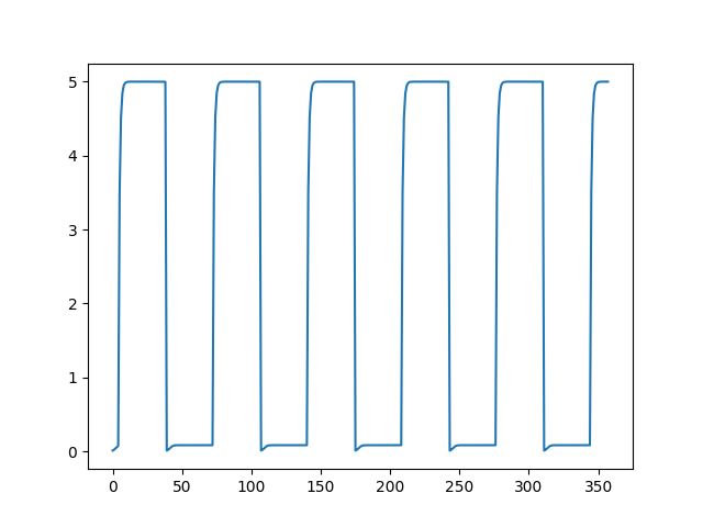 { width=300px }
DT = 0.01
VOLTAGE = 5
R_COLLECTOR = 470
R_BASE = 47000
CAP = 0.000010

c = Circuit()
top = c.new_var()
o1 = c.new_var()
o2 = c.new_var()
b1 = c.new_var()
b2 = c.new_var()
i = c.new_var()

c.new_component(VoltageSource(VOLTAGE, c.gnd, top, i))
c.new_component(Resistor(R_COLLECTOR, top, o1))
c.new_component(Resistor(R_COLLECTOR, top, o2))
c.new_component(Resistor(R_BASE, top, b1))
c.new_component(Resistor(R_BASE, top, b2))
c.new_component(Capacitor(CAP, o1, b2))
c.new_component(Capacitor(CAP, o2, b1))
c.new_component(Bjt(1 / 0.026, 1e-14, 10, 250, b1, o1, c.gnd))
c.new_component(Bjt(1 / 0.026, 1e-14, 10, 250, b2, o2, c.gnd))

solver = c.solver(DT)

duration = 3  # Seconds

points = []

while solver.t < duration:
    solver.step()
    points.append(o1.value)

plt.plot(points)
plt.show()
Alternating vs Direct current
How diodes can convert AC to DC
When capacitors finally become useful
If electrical current is analogous to a ball falling from a higher height, then capacitors are like springs on the ground. When the ball hits the spring, in the very first seconds, you won’t see a fast change in the speed of the ball (capacitor acts like a wire, in the very first milliseconds ). As time passes and the ball pushes the string, the string will get potential energy, slowly preventing the ball to squeeze the spring further. There is a moment where the potential energy of the ball gets equal with potential energy of the spring (capacitor), and that’s when the ball (current!) stops moving. The longer and stronger the spring is, the more it takes to fully squeeze it.
In this fancy, not fully accurate analogy, we can also assume that air-resistance is pretty similar to a resistor. It will slow down the ball. Together, the air resistance and the spring will make a mechanical RC circuit, higher air resistance will also increase the time needed for the spring to get fully squeezed.
Now, imagine we suddenly remove the gravity from the equation, the energy stored in the spring will be released and will push the ball to higher heights, just like when we disconnect the batter from the capacitor and let it load a LED!
Capacitors are DC blockers!
Controlling the world
\(u(t)=K_pe(t)+K_i\int_0^t{e(\tau)d\tau}+K_d\frac{de(t)}{dt}\)
Make it real!
Manufacturing has always been a mystery to me. My most important question always was, how do manufacturers turn any kind of material to the shape they want? How do they automate the process to mass produce stuff? I never got a completely convincing answer, because some of the techniques companies use to shape material and mass produce them is kind of their intellectual property, and you can’t find a lot of resources (At least, on to the point and understandable ones) on the internet! Software engineering is a lazy kind of engineering. There is a magical, general-purpose machine that can do literally anything you want for you. That’s not the case with other kinds of engineering.
Over the years, laziness of software engineers turned to be a good thing for the for the industry too. People started to use software to describe the way they wanted to shape materials (Computer-Aided Design or CAD softwares) and software engineers fetish of abstraction and general purposeness has now inspired building machines that can concert solid blocks into extremely complicated parts for us.
Nowadays, car engines, rocket engines, gearboxes and many other kinds of complicated materials has now got much simpler to produce thanks to the invention of computer sculpturers. Not only easier, but also extremely more accurate!
In this section, we are going to discuss and learn about CNC milling machines and 3D printers, the silicon-valley style of manufacturing stuff!
To add or to remove? That’s the question
There are two main ways to build a shape out of some material. You either:
-
Take a solid, cubic like piece of material, and start cutting it until you get the shape you want. Just like sculpturing
-
Add very small amount of material, little by little, layer by layer, until you get the shape you want.
Which one is simpler? Which one has fewer waste?
As a human, which one is simpler? Definitely the second one. Almost all complicated hand-made materials throughout the history has been made by subtractive manufacturing.
It’s crucial for us to visualize what is happening in our 3D printing simulator in order to see if it is working smoothly, so we perhaps need a 3D rendering library for doing so. We definitely can use our codes in chapter 3 for this reason, but let’s just keep it simple and use a more efficient, production grade library for this purpose. We already know how 3D rendering works so we are not cheating! Here I’ll be using a OpenGL binding for Python named PyOpenGL in order to draw simple boxes. In order to keep the dependency of this book to auxiliary Python libraries as low as possible, I’m going to define an abstracted interface over a 3D rendering library and use that instead of directly calling the OpenGL functions in the codes.
class RenderingLibrary:
    def clear():
      pass
    def draw_box()
      pass
    def draw_sphere()
      pass
Our library will have 3 simple functions, one for clearing the screen, one for drawing a cube and one for drawing an sphere. It by default has some lighting to make the output image feel more 3D. We don’t care how the interface is implemented, but we’ll use it in our code. A working implementation will be provided in the git repo of the book!
I unfortunately didn’t find any article explaining how G codes are generated from CAD files, but here are some guesses and intuitions of how it really works. Never be scared of designing challenging stuff all by your own, that’s where true creativity resides!
The language for communicating with both subtractive and additive manufacturing machines is a computer language named G code. Although it’s referred as a programming language, it really isn’t. It doesn’t let you have loops, conditions and etc. it only lets you to move the extruder or the mill to arbitrary locations!
G code is a big language and has a lot of commands, so simulated 3D printer and CNC machine will use a subset of G code, only including the most important commands.
Our goal in this section is to generate G code commands for building a 3D sphere in both additive/subtractive manufacturing machines. We also want to see the outcome of those two using our RenderingLibrary.
In order to make things simpler, let's just assume that our model accepts 5 tokens as input and gives out the next predicted token as output. Just like how we built a model that was able to learn MNIST and XOR, we can take the most naive approach and build a multi-layer-perceptron. But there is something really very wrong with this approach when trying to build something like a chatbot. Let me explain it to you with an example. Imagine the sentence you are going to process and predict its next word is something like this:
"I'm called Keyvan, so my name is"
The word "Keyvan" is a great example of a word that we most probably have not reserved an independent token for. If you take a large piece of english text and sort the words appearing in it by number of occurance, "Keyvan" is definitely not in the first 1000, but since a token-embedding should be able to decompose any word into a list of tokens, it's probable that the word Keyvan will be decomposed to "Key", "v" and "an".
Now, based on this, it's obvious that the next token that should appear after "I'm called Keyvan, so my name is", should be "Key". But, think about it, is a multi-layer-perceptron really able to efficiently learn to predict something like that? This is what the neural network have to do:
- Ignore the fact the word "Key" has a meaning on its own.
- Find the token/tokens that are related to the name of the person.
- Copy those tokens one by one, and keep track of tokens it has already copied.
You can experiment it. Build a neural network as deep as you want. It will struggle to learn something as simple as that, very badly.
The solution? Well, you can again try to get inspiration of how your own brain really works. When you try to recall the name of someone, your brain will start looking for very specific parts of your memory, your brain will stop caring about every other piece of your memory and will try to replicate the only parts of your knowledge that matter. In terms of a neural network that predicts the next word of a sentence, sometimes all you need is a look-up in the sentence and in that case, the neural network should be able to dynamically figure out the words that matter the most when predicting the next word. Without such mechanism, your neural network will give equal opportunity to all of the tokens in your sentence to participate in the prediction of the next token, and our neural networks are limited in size.
As a result of a research done in 2017, the researchers discovered a beautiful method for allowing neural networks to pick the most relevant pieces of data as the input goes through the model. They named it "Self-Attention" or "The Attention Mechanism", or "The Transformer Architecture". The title of their paper is also "Attention is all you need", and it really turned out that attention was all we needed! The idea is very brilliant:
Imagine you are in a room, full of people talking, and you want to ask some question from a friend...
The non-trivial gate, XOR
A non-trivial way to search
The Transformer model tries to emulate some kind of database within a neural network, but before trying to play with neurons, let's discuss the non-neural-network version of it:
import math

database = [
    ([0.52, 0.78, 0.69], [0.29, 0.51, 0.17]),
    ([0.45, 0.54, 0.12], [0.63, 0.49, 0.91]),
    ([0.14, 0.59, 0.53], [0.52, 0.46, 0.25]),
    ([0.79, 0.96, 0.91], [0.32, 0.32, 0.17]),
    ([0.01, 0.73, 0.69], [0.68, 0.73, 0.75]),
]

keys = [k for k, _ in database]
values = [v for _, v in database]


def closeness(a, b):
    eps = 1e-5
    ret = 0
    for x, y in zip(a, b):
        ret += (x - y) ** 2
    return 1 / (math.sqrt(ret) + 1e-5)


def softmax(inp):
    max_x = max(inp)
    e_x = [math.exp(x - max_x) for x in inp]
    sum_e_x = sum(e_x)
    return [x / sum_e_x for x in e_x]


to_find = [0.79, 0.96, 0.91]
dists = softmax([closeness(k, to_find) for k in keys])

res = [0, 0, 0]
for k, v in zip(dists, values):
    for i in range(3):
        res[i] += k * v[i]

print(res)
The difference between this creative way of searching, and a regular search is very similar to the difference between a neuron, and a logic gate. One of them is differentiable, and the other is not!
A hard, solid piece of rock is a creature that perhaps doesn't experience any of the human feelings. A rock doesn't fall in love, or become happy or sad. A rock will experience no pain, doesn't need to breath and eat to survive, you might think that a rock has a wonderful life (And in some ways, it has).
A rock's luckiness perhaps partly comes back to the fact that it has a fairly simple structure. If you study the molecular structure of a rock, you will see that a rock is built of a limited set of atoms, orderly placed along each other, which makes it a very hard break. A human being on the other hand has a much more complicated structure, and we can't see the perfect atomical ordering of a rock in a human body too. While a rock has a wonderful life, its life is very boring (From the viewpoint of an observer), a human life on the other hand, despite having sadness, pain and suffer, is much more interesting and worth living. Nature's goal has never been to build a long-lasting life, without any happiness and pain like a rock, but to build a life that maximizes interestigness.
You might now already know that I'm going to talk about one of the most interesting laws of physics, the second law of thermodynamics. This law was first discovered by Sadi Carnot, the french Physicist, who discovered that you can't build a motor engine that is able to convert 100% of the heat energy into mechanical work, and some of the energy will always be wasted. In other words, there is a efficiency limit in a system that converts heat into mechanical work. The same law can be expressed in other ways too, for example, you can't build a refrigerator (Or an air conditioner) that is able to decrease the temperature of a closed area, without disposing a higher heat (Higher than the amount reduced in the closed area) outside that area.
Heat is some kind of chaos and disorder in atoms. When atoms take energy, they start to move in directions in a chaotic way. The more they move, the hotter they become. We can measure how chaotic the elements of a system (E.g. the atoms inside a closed area) are, and call it the Entropy of that system.
Given the definition of Entropy, we can redefine the second law of thermodynamics in another words: The entropy of the universe always increases. I.e the sum of disordered-ness of all elements in our universe always gets higher, which again means, I can't decrease the heat in my room in a sunny day without generating even more heat into the universe. You might now think that we are making the earth warmer by building air conditioners, but the truth is the heat is radiated into the universe!
Maybe?
- See - Pattern recognition in images
- Build - C compiler
Appendix A
When your program becomes alive!
Writing a C compiler in C